In this case, z is a parameter you need to set to 1 in steady state.
Is it possible to do the same with the rest of shock variables (x, a, e, v)?
For example, in
k(+1)=(1-delt)*k+x*in,
if I try to express delt I get
delt=(x*in)/k,
which will be again 0, because x is a shock assumed to be zero in the steady state (I assume k(+1)=k). I want to emphasize that z is a variable, not a parameter, but I guess this is irrelevant or it can be treated as a parameter.
The steady state of exogenous variables is indeed a parameter you can fix to 1.
I obtain unusual data, when trying to compute parameters from the model equations. For example, for et = lambd * w * (1-h) I obtain 7161994 instead of 1.5 suggested by literature. Eta is a relative weight of leisure, entering household’s utility function
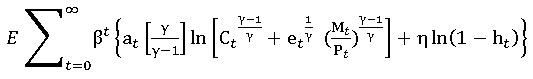
But when e.g. h (number of working hours in year, set to 1834) and w (yearly wage, set to panel average 13124) are entered, value immediately increases.
Another question, would it make more sense to first try to make calibrated model work before introducing it to the real world data? I read this on DSGE parameters - #2 by DoubleBass What could I enter then instead of real world data for consumption, investment etc. to make estimation work?
Model.mod (1.7 KB)
Model_steadystate.m (1.1 KB)
Your utility function is only valid for the share of hours being normalized to 1. Your leisure is 1-h_t after all. That explains the different numbers. Similarly, you cannot just plug in a number for the wage without adjusting TFP accordingly. That’s why a model needs to be carefully calibrated.
What real world data could I use as a scaling variable?
I’ve seen labour productivity (technology shock used by Christiano or “level of technology” by Fernandez-Villaverde) used in this role rather than TFP, but I may be wrong.
With constant returns to scale, the scaling is arbitrary. Only ratios matter. For that reason, most researchers normalize TFP to 1 and hours worked to something like 0.33 and work from there.
Thank you for answer, I understand. I intend to set hours worked to number of working hours in year 1834 divided by all hours, i.e. 0.21 or use 0.33. But wage and other non-stationary variables should probably also be adjusted somehow? I mean, if I divide wage 18341 by TFP 1, there’s probably no way I’m getting et 1.5 instead of 7161994 according to the equation above.
What is your calibration target for \eta?
It’s 1.5.
But what is the meaning if that 1.5? It’s usually a ratio of something to something.
It means household’s labour supply in the steady state amounts to one third of its time.
But for that type of calibration you don’t need any data.
OK, I understood that parameter values are computed out of the steady state equations by inserting variable data. We mentioned this in posts #52 and 53. So how else would I compute the parameters if not from steady state equations?
I don’t understand where exactly your problem is. Of course the parameters are set based on the steady state equations and calibration targets. But the usual targets are scale-invariant, i.e. they are ratios that do not depend on e.g. the level of TFP or the level of the wage.
But how else would I compute the parameter out of the steady state equation, if I don’t enter the e.g. level for wage? For example in formula for eta, et = lambd * w * (1-h), I entered 0.33 for h, -0.41 for lambd and 18341 for wage.
Given the other parameters and your calibration targets, you can compute w and lambda from the model.
It seems I was approaching calibration from the wrong side. It’s about inserting parameters/calibration targets in order to compute steady state variable levels, and not inserting variables in order to compute parameters.
That said, plugging in the parameter values, I still obtain a rather complex system of 20 equations, that can’t be solved by hand, so I have few questions.
- My equations contain variables in specific time period t, as well as a steady state value, e.g. r_t and r in a Taylor rule:
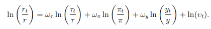
I designated this as r and r0 in the model, adding extra 6 equations in which I determine e.g. r0=8.88;, based on my real world observations. Is this a correct way, or could I simply insert observed values in the equations now when computing parameters?
- In several equations I have variables in different time periods, e.g. k(+1)/k. You told me this can be simplified to k(+1)=k in a steady state only in a detrended model, so I wonder if I have to divide the expression with TFP in order to do it and how could I compute the TFP (works of Christiano and Eichenbaum don’t mention how to compute the scaling factor in practice).
System of equations.txt (1.6 KB)
- The Taylor rule only states that all variables will be at their steady state value in steady state, given your desired steady state inflation rate. That rate can be fixed. The relevant other equation is the Euler equation, which will pin down the real interest rate based on the discount factor.
- Most models are already written down in detrended form. They then feature terms like (k_{t+1}/k_t-1) instead of (k_{t+1}/k_t-\gamma_k)
Excellent, so if I understand correctly I can delete six equations for the steady state variables, and keep original 20 equations only, with steady state values inserted.
After simplifying terms k(+2)=k(+1), i obtain some results that don’t seem right. The first result I obtain numerically is q=-0.975 out of equation
lambd*(32.14*(k(+1)/k-1))=0.99*(lambd(+1))*((q(+1))+0.975))-15.91*(lambd(+1)*(k(+2)/k(+1)-1)^2)+0.99*phik*lambd(+1)*(k(+2)/k(+1)-1)*(k(+2)/k(+1));
The negative values then spread as I plug q in other equations to obtain lambd=-0.327 and w=-6.881.
System of equations.txt (1.3 KB)