Help Needed: DSGE Model Bayesian Estimation

Hello everyone,

I’m facing a challenge with my DSGE model estimation in Dynare and would appreciate any insights from the community. My model works well with the stoch_simul command, but I encounter issues when using Bayesian estimation.

Currently, I can only successfully estimate the model with the following four observables:

y_us_obs, smdi_obs, real_price_silver_obs,real_exch_obs

However, my model has seven shocks, and I recall that, in theory, the number of observables should ideally match or exceed the number of shocks for full identification. This discrepancy raises concerns for me regarding the accuracy of the estimation results, as I’m working with fewer observables than shocks.

When I attempt to add more observables (such as pc_A_obs for agricultural value index, pc_N_obs for non-agricultural sector price index, y_obs for output, m_obs for money supply, im_obs for imports, and xp_obs for exports), I receive the following error message:

initial_estimation_checks:: The forecast error variance in the multivariate Kalman filter became singular.
initial_estimation_checks:: This is often a sign of stochastic singularity, but can also sometimes happen by chance
initial_estimation_checks:: for a particular combination of parameters and data realizations.
initial_estimation_checks:: If you think the latter is the case, you should try with different initial values for the estimated parameters.

ESTIMATION_CHECKS: There was an error in computing the likelihood for initial parameter values.
ESTIMATION_CHECKS: If this is not a problem with the setting of options (check the error message below),
ESTIMATION_CHECKS: you should try using the calibrated version of the model as starting values. To do
ESTIMATION_CHECKS: this, add an empty estimated_params_init-block with use_calibration option immediately before the estimation
ESTIMATION_CHECKS: command (and after the estimated_params-block so that it does not get overwritten).“

To preprocess my data, I use Stata to: 1. Log-transform and then difference each series; 2。 Detrend each differenced series to ensure a mean of zero.

My understanding is that the issue might be stochastic singularity due to potential collinearity among the observables. However, even if I add a single, seemingly independent variable, such as pc_A_obs (agricultural product price), which should not be collinear with variables like foreign output and exchange rate, I encounter the same error.

I also suspect that parameter dependence could be contributing to the issue. I read A Guide to Specifying Observation Equations for the Estimation of DSGE Models by Johannes Pfeifer, where parameter dependence is discussed, but I’m uncertain if this applies to my case. In particular, I’m concerned about the piz and bG variables. I attempted to define these with # to handle dependence, but this resulted in the following error:

piz has wrong type or was already used on the right-hand side.

Could anyone offer guidance on:

  1. Whether having fewer observables than shocks in the current model setup could lead to unreliable estimates?

  2. How to effectively identify and resolve any parameter dependence in piz, bG, or other variables, and whether this is indeed the root cause? The problem may arise from other issues??

  3. Suggestions for handling the stochastic singularity problem, especially regarding the addition of more observables?

Thank you in advance for any advice you might have.

Best regards,
Yamoi
model_sim_bayesian.mod (26.2 KB)
data1911_19364.xlsx (7.3 KB)

param_and_ss_10_25.m (5.7 KB)
  1. You can have at most as many observables as shocks. Having fewer observables is typically not an issue.
  2. Your model looks like it should have a steady state file. That would also take care of the parameter dependence.
  3. You should try to find out where the stochastic singularity comes from. There must be an exact linear combination hidden in your model.

Hi Prof. Pfeifer,

Thank you very much for your response!

“You should investigate the source of the stochastic singularity, as there must be an exact linear combination hidden within your model.”

Could you let me know how to identify this, apart from using the model diagnostic tool? Or is the model diagnostic tool the only available method?

Best,
Yamoi

I am not aware of any additional technique. Most of the time, it’s about looking at the model equations again to understand what is happening.

Thanks for the advice.

Yamoi

Hello everyone,

I have a few questions related to setting up shocks, data configuration, and estimation in my DSGE model, and I’d really appreciate your insights on the following points:

  1. Shock Timing
    In my model, I have specific shocks occurring at different points in time:

The natural disaster shock (eta_eC) occurs in 1931 and 1934.
The foreign consumption shock (eta_c) occurs in 1929.
Shocks to international silver price (eta_pws), international gold price (eta_pwg), and domestic silver price (eta_pds) occur in 1929, 1931, and 1934.
The productivity shock (eta_z) is estimated via Bayesian methods, so the timing is not explicitly known.
Since Bayesian estimation already estimates the shock sizes for variables like sig_c, sig_g, etc., is it necessary to specify the timing for each shock manually? If so, how can I set different timing for each shock in Dynare?

  1. Setting presample and first_obs
    My data covers 1911 to 1935, but my primary research focus is on the economic period from 1929 to 1935. The data is in an Excel file, with the first row as variable names. The actual data starts from the second row, making 1929 data appear in row 20 (or row 19 if the first row of names is excluded).

I’m currently considering presample=0 and first_obs=2, which would use all data from 1911 onward. However, I’m concerned this might dilute the focus on the 1929-1935 period. Do you think setting presample=0 and first_obs=2 would still allow me to capture the 1929-1935 period effectively, or should I adjust these settings differently? Any advice?

  1. Specifying Shock Correlation
    I know that eta_pws and eta_pwg have a high correlation of approximately 0.52. I wanted to define a parameter (corrpwsg) to represent this correlation, then estimate it within the model. My idea was to define the correlation as follows:

dynare
Copy code
corr eta_pws, eta_pwg = corrpwsg;
I assigned an initial value to corrpwsg and attempted to estimate it under a Beta distribution in the estimated_params block. However, this setup caused errors during runtime. Is there a way to correctly define and estimate a correlation parameter between shocks in Dynare?

  1. Shock Identification and Independence in IRFs
    I have seven shocks in total in my model. Should I perform identification checks for each shock to ensure that they are identifiable? Additionally, when I run impulse response functions (IRFs), are these shocks considered completely independent of each other in Dynare, or do I need to specify any further assumptions?

Thank you very much for your time and assistance. Any guidance you could provide on these issues would be greatly appreciated.

Yamoi
model_sim_bayesian10_31.mod (30.7 KB)

  1. Bayesian estimation in Dynare is not well-equipped for estimating one-time discrete shocks. They are more like structural breaks. What you can try is using the heteroskedastic_shocks-block to shut off these shocks in other periods. Of course, only observing a one-time shock makes identifying them hard.
  2. Having a longer sample should allow you to better estimate the parameters. However, if you think the period before 1929 was structurally different, you should use it as the presample. That would essentially use these observations to update the prior, but they will not enter the likelihood.
  3. Correlations can be directly estimated in the estimated_params block.
estimated_params:
corr eta_pws, eta_pwg, .... beta_pdf, ...;
end;

See the manual.
4. Yes, shocks are independent unless there is specified correlation. In that latter case, Dynare will use a Cholesky decomposition to orthogonalize shocks. Again, see the manual. And yes, checking identification is a good practice, though complicated by the need to use heteroskedastic_shocks.

Hi Professor Pfeifer,

Thank you for your earlier advices—That was very helpful. Following your suggestions, I have successfully generated prior distribution graphs for my parameters. However, I am still facing one issue with my model file:

  1. Defining Correlations between Shocks: I also encountered an error when attempting to set a correlation between eta_pds and eta_pwg using:

corr eta_pds, eta_pwg, beta_pdf, 0.5, 0.2;
Including this line (on line 382) leads to errors

“ERROR: model_sim_bayesian11_05.mod: line 382, cols 35-42: syntax error, unexpected BETA_PDF, expecting ‘;’”

I’ve attached the full .mod file for your reference.

Thank you for your time and support.

Best,
Yamoi
model_sim_bayesian11_05.mod (28.9 KB)
param_and_ss_11_05.m (7.0 KB)
~$data1911_19364.xlsx (165 Bytes)

You forgot the initial value. Use

    corr eta_pds, eta_pwg, 0,		,		, beta_pdf,			.5,           	0.2;

Oops… now it works. Thanks!

Hi Prof. Pfeifer,

I’m working on a DSGE model to analyze the impact of the U.S. Great Depression on China’s economy during the period from 1929 to 1935. I’ve set up my code as follows to use data from 1912 to 1935, with a presample (1912-1928) included so that the model uses information from before the crisis period.

Here’s the code I’m using:

"
estimation(order=1,
datafile=‘data1911_19364.xlsx’,
presample=18,
first_obs=1,
prefilter=0,
plot_priors=1,
lik_init=2,
mh_nblocks=2,
mh_jscale=0.38,
mh_replic=1000000,
mode_compute=6,
mh_drop=0.1,
nodiagnostic,
moments_varendo,
bayesian_irf,
irf=20,
mh_conf_sig=0.95,
conf_sig=0.95);
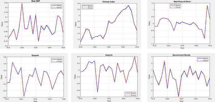
presample =18 means (from 1912-1928 in my excel data). The problem I’m facing is that the estimated values align almost perfectly with the actual data for all variables, which seems too good to be true. I’m concerned that the model might be overfitting the data or not capturing realistic forecast errors. My understanding is that by including the presample data (1912-1928), I think the model should ideally use this historical information (1912-1928) to forecast 1929-1935 if I want to study the impact of great depression on China(1929-1935), right? Or Is my understanding wrong? yet the current results show almost no deviation between the model’s predictions and the actual values.

My questions are:

  1. Do you think the attached results are too good to be true? Could this setup lead to overfitting, where the model tracks the actual data too closely? To achieve my goal, how to correctly set up the code? What adjustments might help?

  2. Is the forecast command appropriate for evaluating out-of-sample errors in this setup, and would it be helpful here?

Any insights or suggestions for fine-tuning this setup to ensure more realistic forecasts would be greatly appreciated. Thanks in advance for your help!


data1911_19364.xlsx (17.4 KB)

Thank you!

Best,
Yamoi

I am not sure I understand. Full information estimation techniques by construction replicate the observed data (except for measurement error).

Hi Prof. Pfeifer,

Thanks for the response. I am currently working on a historical economic analysis related to the impact of the Great Depression (1929-1935) on China. I am trying to understand the best way to implement two estimation approaches in Dynare and would appreciate your insights.

Reference Example:
In my research, I came across an article that studied the impact of the pandemic shock on inflation. They mentioned their estimation approach as follows:

Our estimation makes use of U.S. data for the period 1983:Q1-2019. Therefore, we do not include the pandemic episode in the estimation. The rationale behind this choice is to show that a model that is estimated using pre-shock data can predict the dynamics of inflation and labor market variables once a shock, such as the one that we describe in this paper, hits the economy. We then set the standard deviation of the shock to match the rise in the unemployment rate during the first quarter of the pandemic. That would be the only target that we match since March 2020. We also acknowledge that the sample period since the start of the Covid-19 pandemic is relatively short, which limits our ability to rely solely on this period for estimation (at the time of this writing, we have only 11 quarters of data available for certain variables). In the Appendix, we present results based on data that also includes the pandemic period (1983:Q1-2022).

My Questions related to my research:

  1. Understanding the Differences: I am trying to understand the differences between using full information data (e.g., 1912-1935) for estimation versus estimating the model with pre-shock data (1912-1928) and using it to predict macroeconomic variables during the shock period (1929-1935). Why might one approach be preferred over the other, and what potential biases or limitations should I be aware of when using full information estimation?

  2. Code Implementation: Based on my understanding, I have drafted two code structures in Dynare:

The first way:
Pre-Shock Estimation (1912-1928) with Forecasting (1929-1935):

estimation(order=1, 
           datafile='data_1912_1928.mat',  
           first_obs=1, 
           prefilter=0, 
           plot_priors=1, 
           lik_init=2, 
           mh_nblocks=2, 
           mh_jscale=0.38, 
           mh_replic=1000000, 
           mode_compute=6, 
           mh_drop=0.1, 
           nodiagnostic, 
           moments_varendo,
           bayesian_irf, 
           irf=20, 
           mh_conf_sig=0.95, 
           conf_sig=0.95);

// Forecast shocks for 1929-1935
forecast(nobs=7);

After the forecast, how to find the estimated data for period 1919-1935 and compare the estimated data with real data?

The second way:
Full Data Estimation (1912-1935):

estimation(order=1,  
          datafile='data1911_1935.xlsx',  
          presample=18, // Optional: to omit initial observations before 1929 if needed
          first_obs=1, 
          prefilter=0, 
          plot_priors=1, 
          lik_init=2, 
          mh_nblocks=2, 
          mh_jscale=0.38, 
          mh_replic=1000000, 
          mode_compute=6, 
          mh_drop=0.1, 
          nodiagnostic, 
          moments_varendo,
          bayesian_irf, 
          irf=20, 
          mh_conf_sig=0.95, 
          conf_sig=0.95);

I am wondering which one is correct, or if neither of them is correct.

Additional Questions:

  1. If the first way is better, should I still need the presample option for these historical estimations, or is it unnecessary given the period I am studying?
    Is using forecast(nobs=7) the best way to analyze the 1929-1935 period, or could the original estimation with the full dataset be sufficient?

  2. How can I check if a model is overfitting? If I use full information with data from 1912-1935, and the estimated data and real data are almost perfectly aligned (see the graphs in my last post), does this indicate overfitting?

  3. How can you determine if a model is good or not?

  4. In Bayesian estimation, I am wondering what exactly is being targeted. Are we estimating the mean, variance, correlation, or something else?

My understanding is that Bayesian estimation aims to estimate the posterior distribution of model parameters, which includes the mean, variance, and potentially the correlation among parameters. Is this correct, or is there more to consider?

Any guidance or insights you could provide would be greatly appreciated. Here is the paper I referred to if needed (the details of their estimation are at the bottom of page 16). https://simon-xg-sheng.github.io/web/working%20paper/Inflation_LaborMarket_Sept5_2024.pdf.

Thank you for your time and help!

Best regards,

Yamoi

As your goal is still not clear to me, I cannot comment on which approach is correct. My hunch is neither. The paper you reference estimates the model on pre-Covid data because it assumes that the structure of the economy has stayed the same after 2019, only the shocks have become bigger. It then does IRFs keeping the parameters at their old value, but with a larger standard deviation for the shocks. That seems different from what you are trying to do.

  1. Option 1 would be forecasting data without any shocks occurring in the second period. That seems inconsistent with what you are trying.
  2. The point of full information estimation is to perfectly fit the observed data. After all, you assume the model is the data-generating process.
  3. and 4.: A good starting point is How to see whether the model fit the real data well? - #2 by jpfeifer

Hi Prof. Pfeifer,

After further reflection, I revised my question and made it shorter for clarity:

If the economic structure after 1929 changed due to the Great Depression, estimation should use pre-1929 data for priors, while 1929–1935 data should enter the likelihood. However, if the structure after 1935 differs again (e.g., due to war), forecasts starting in 1936 would be unreliable. Is this correct?

Alternatively, if I assume the economic structure is consistent throughout 1911–1935, I could estimate the model using all data (including 1929–1935) without needing a presample. In either case, including 1929–1935 data in estimation is valid since it’s a full-information approach. Does this understanding make sense?

Thank you!

Best,
Yamoi

Yes, that is correct and makes sense.