Help: Filtering differences Matlab vs Dynare

[colenso2000]

Hi all,
I’m exploring Dynare’s filtering capabilities through a simple exercise: I take a basic state-space model, apply MATLAB’s smoother to recover the smoothed states, and compare the results to those produced by Dynare. The state-space model is based on the policy function of a neoclassical growth model, using the calibration provided on page 19 of Uhlig’s toolkit, and assumes no measurement error and has one 1 observable (PCE). The data file for Dynare is log_deviation_data.csv.

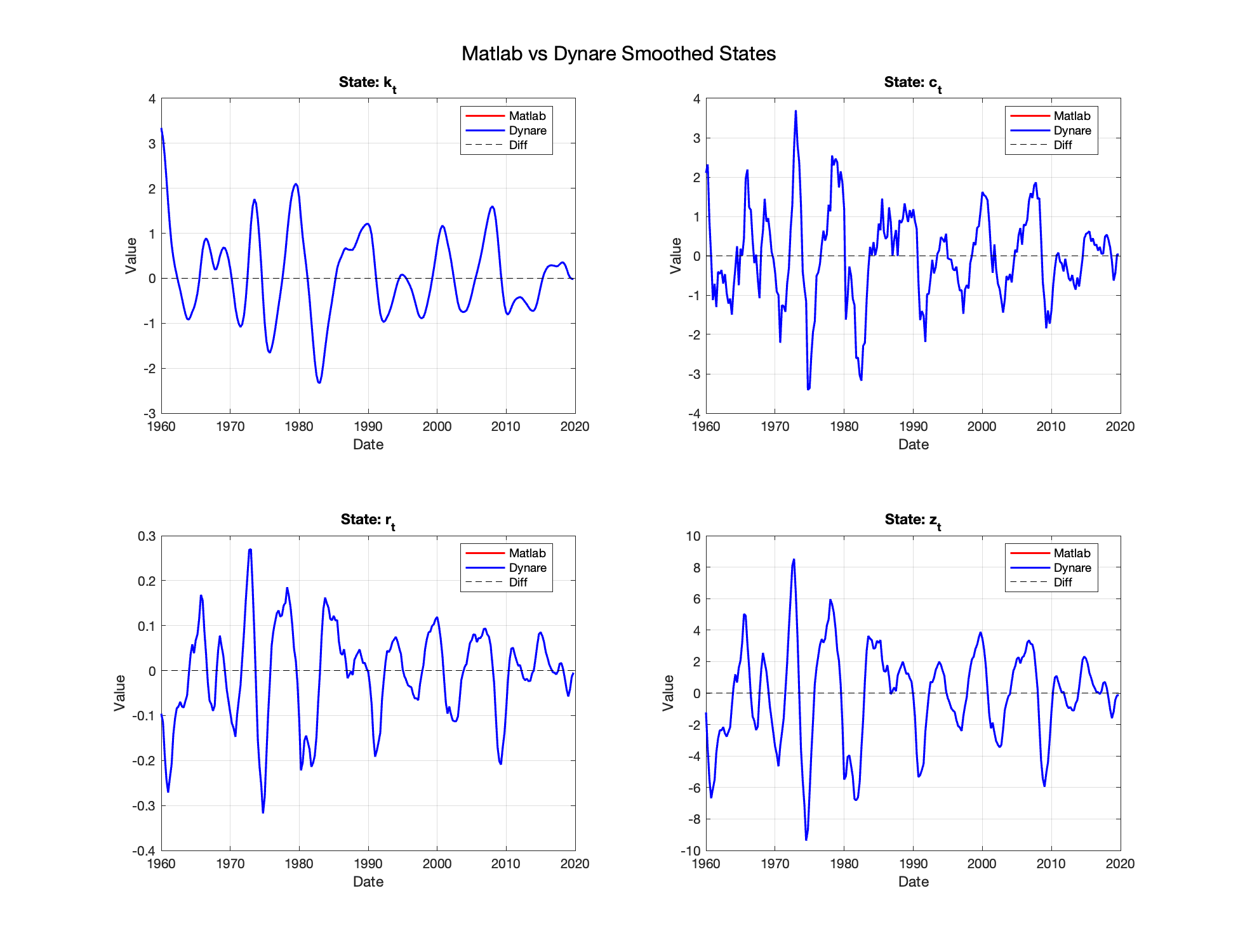
I provide Dynare with the same model and calibration, using “mode_compute=0” to bypass estimation. I also give the two models the same initial assumptions for the states (S_0 and P_0). However, aside from the one observed state, I get noticeable differences between the series produced by MATLAB and those generated by Dynare (see image below).

The files “example_ssm.m and ParamMap.m” generate the smoothed series using Matlab’s KS. The file “try_1.mod” is Dynare’s mod file. Finally, “try1_comp.m” compares results and plots the series and their difference. I’m running Dynare 5.5:

log_deviation_data.csv (4.3 KB)
example_ssm2.m (4.0 KB)
ParamMap.m (1.0 KB)
try1_comp.m (1.3 KB)
try_1.mod (2.0 KB)

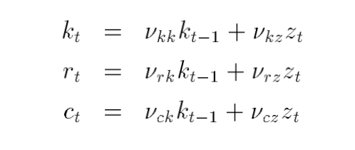
The problem appears to be the transition matrix A, where it should be:
A = [ 0.965, 0, 0, 0.07125;
0.618, 0, 0, 0.28975;
-0.022, 0, 0, 0.03325;
0, 0, 0, 0.950];

(as in the Matlab file), in Dynare it is being populated as:

A = [ 0.965, 0, 0, 0.07125;
0, 0.618, 0, 0.28975;
0, 0, -0.022, 0.03325;
0, 0, 0, 0.950];

I guess that I’m overlooking something in the model description, but I haven’t been able to identify what it is. Any help would be greatly appreciated @jpfeifer. Thank you!

[jpfeifer]

I am not sure I understand what you are doing here. You are not solving the model in Dynare but rather entered a backward-looking model. In any case, there are related threads:

IRFs from the ABCD state space representation

Hi everyone, I was thinking to quickly compare the IRFs produced by dynare with the ones of the state space retrieved from the ABCD test (to make sure everything is correct). For the latter I used the integrated IRF MATLAB function for state spaces. For the IRF comparison I just used an older model of mine. As you will see there’s a big difference between dynare’s and the “my computation”. If you just run the “compare_irfs.m” file you get the relevant plot. Most probably I can’t just use the A…

[colenso2000]

Thank you @jpfeifer. Essentially, I’m providing both MATLAB and Dynare with the same policy functions for a neoclassical growth model (specified below) and using the same data to obtain the smoothed states via each platform’s smoother:

I have 4 unobserved states (k_t, c_t, r_,t and z_t) and 1 observable (c_t). I noticed that in my original mod file, I had a typo where c_t and r_t were not depending on the state variable, capital. After fixing that, the smoothed series are now a perfect match.

try_1.mod (2.0 KB)

While this is encouraging, I have two short doubts:

1. What is the interpretation of “oo_dr.ghx”? I believe this must somehow map into the state transition matrix A, but I cannot understand how. In the current version of the mod file, I’m getting
   oo_dr.ghx"= [ 0.6180, 0.28975;
   -0.0220, 0.03325;
   0.9650, 0.07125;
   0.0000, 0.95000];
   which does not even match the dimension that I was expecting for the transition matrix.

Something similar happens with oo_dr.ghu", which I’m guessing somehow maps to B. While the dimension in this case is as expected, the numbers are not when compared to the B matrix in the Matlab specification of the SSM:
oo_dr.ghu = [ 0, 0.305, 0, 0;
0, 0, 0.035, 0;
0.075, 0, 0, 0;
0, 0, 0, 1];

2. While the smoothed series are identical, the computed likelihoods are not that close. Dynare is reporting that the initial value of the log posterior (or likelihood) at -397.839, while Matlab is reporting the likelihood at -270.28. Is this difference somehow to be expected?

Thanks again!

[colenso2000]

A small correction to my previous update: initially, I had defined four exogenous variables for each error term (ek, ec, er, and ez), but there is only one shock in the model (z) and one exogenous variable (ez). In my MATLAB’s SSM this is done correctly. After making this adjustment in Dynare, small differences between the smoothed series reappeared. What is the correct Dynare syntax to use in this case? If the single shock is the right way to do this (see “try_2.mod”), what could be driving the differences?

try_2.mod (1.9 KB)

I also noticed that the parameter SIGMA was not being picked up by Dynare’s smoother. One workaround is to include the parameter directly in the model equations (e.g., SIGMA * ez), which allows me to see changes in the parameter values reflected in oo_.dr.ghu. I was wondering whether this issue is due to using the mode_compute = 0 option, or if it’s simply because the shocks block isn’t necessary unless stoch_simul is used.

Thanks again for any help and guidance.