Hello Dynare comminity,
Recently I got interested in using HANK models for non-linear fiscal multipliers. But the problem lies in practical part of it.
I came across few sources of codes which solves the HANK model in Dynare. First is Thomas Winberry’s codes ( which I found on Dynare forum) and another one is presentation by Normann Rion and Sébastien Villemot (/https://sebastien.villemot.name/pdf/talks/2024/hank.pdf). Which also includes codes in Dynare.
In both cases I failed to successfully execute those codes in Dynare.
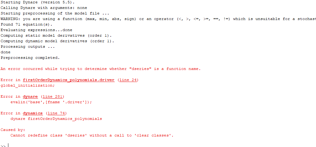
As for Thomas Winberry’s codes, the dynamics.m file runs into the error.
As for Normann Rion and Sébastien Villemot case, when trying to write it as a model (from codes given in presentation, but I could not fully build all blocks of model from the presentation) using latest stable Dynare. But I am not quite sure the commands given in presentation are yet implemented in Dynare. If so can someone help me on this issue to finish the all blocks of the model for HANK model (I am attaching the model file).
Thanks in advance
HANK.mod (958 Bytes)
Thank you very much for reply professor Pfeifer, looking forward to addition of HANK codes in December.
As for error message for Windberry’s codes here is the snapchat of it
(I tried running it on dynare 5.5 and 6.4 with matlab R2018b).
That very much looks like a path conflict.
(1) is a great development! I have a couple of questions:
What algorithm does Dynare use to solve for the steady state of the model? Time iteration on the Euler equation?
In the example on the slides, Dynare is able to handle a constraint like k’>=0. What about discrete choices like owning vs renting or occupational choice?
Thanks in advance!
@normann can say more about this. The current draft at Draft: Add experimental steady-state computation for heterogeneous-agent models (!2428) · Merge requests · Dynare / dynare · GitLab for solving the steady state uses a solver that:
- Solves the household problem via time iteration to compute policy functions
- Computes the stationary distribution using transition matrices and a forward iteration loop
- Compute the aggregate residuals of equations involving aggregated heterogeneous variables
Discrete choices are not yet supported, I think.
Hi @aledinola13,
Sorry for my late response! Discrete choices are not yet handled natively. One may approach discrete-choice setups by using extreme-value taste shocks.
Note that there is no conceptual reason preventing our resolution method to tackle properly those taste shocks. We may introduce this possibility in the future.
Best regards,
Normann
Thanks for your reply. I was wondering also if there is a document that explains how Dynare solves the steady state of heterogeneous models.
Hello @aledinola13,
I haven’t had the time to write a detailed documentation yet. I plan to do so by the end of the year. The algorithm I use is pretty standard. Let me try to sum it up here.
The key idea is to define a function F(\theta), that takes the free parameters \theta (e.g. beta_ss, vphi, chi1 in hank_two_assets_steady_state.mod) as input, runs the full steady-state computation (phases 1-3 below) for those parameter values, and returns the residuals of a set of user-specified calibration target equations (typically market-clearing conditions involving SUM() operators). Each evaluation of F is expensive, since it requires solving for policy functions, computing the stationary distribution, and aggregating. Dynare then eventually finds one root F(\theta^*) = 0 using a Broyden quasi-Newton solver.
Here are the 3 phases to compute F(\theta).
Phase 1: time iteration (backward iteration on policy functions)
This is the core of the steady-state computation. Starting from an initial guess for the policy functions on the discretized grid, Dynare iterates backward:
- For each grid point (over idiosyncratic shocks and endogenous states), compute expected future policy values via multilinear interpolation on a tensor product grid, using a Gray code algorithm to efficiently traverse the corners of the interpolation hypercube.
- Solve the household’s first-order conditions at each grid point. This is done with a trust-region solver combined with a Fischer-Burmeister transformation to handle inequality constraints (e.g. borrowing limits expressed as complementarity conditions).
- Update the policy functions, optionally with dampening controlled by a learning rate parameter.
- Check convergence: the iteration stops when the sup-norm of the policy update falls below the specified tolerance.
Phase 2: forward iteration on the distribution
Once the policy functions have converged, Dynare computes the stationary distribution of agents over the state space using Young’s method (forward iteration):
- Initialize the distribution uniformly (weighted by the stationary distribution of the exogenous shocks).
- Iterate forward: given the converged policy functions, compute how the mass at each grid point is redistributed to next-period grid points, again using multilinear interpolation via Gray code traversal.
- Apply the Markov transition kernel for the exogenous shocks.
- Repeat until the distribution converges.
Phase 3: aggregation and residual computation
With the converged policy functions and stationary distribution in hand, Dynare computes aggregate variables by integrating the policy functions against the distribution (i.e. evaluating the SUM() operators). It then evaluates the aggregate model equations and returns the residuals of the user-specified target equations. This is the output of the big function F(\theta), which the Broyden solver drives to zero.
Hope it helps!
Best regards,
Normann
Great explanation, thanks! Could you please point to the code that implements Phase 1 (time iteration) of the algorithm described above? Is it written in Fortran with a MEX interface?
Hi @aledinola13,
The source code of the time-iteration algorithm is located in mex/sources/heterogeneity/utils/time_iteration_tensor.f08. It is indeed written in Fortran.
Best regards,
Normann