Generate error bands for IRFs

Hi Professor,

How could I modify the code below to that Matlab could show the 1 unit standard error bands for my each of my IRF subplots?

The data file I am uploading is IRFfull.csv

the code I am using is:

clear all; close all; clc;
load IRFfull.csv;
varname=char('Risk-free rate (r)','Investment (inv)','Tobin''Q (qq) ',...
'Capital (k)','Inflation (\pi)','Wage (w)','Consumption (c)',...
'Output (y)','Labour (l)','Capital Utilisation (rk)',...
'Credit premium (pm)','Risky rate (cy)','Net worth (n)',...
'M0','M2','Unemployment (u)','Export (ex)','Import (im)',...
'Real exchange rate (q)','Foreign assets position(b)');

    for i=1:20
    subplot(4,5,i)   
    plot(IRFfull(:,i),'b','LineWidth',1);	
    axis tight;
    ax = gca;
    ax.YAxis.Exponent=0; 
    title(deblank(varname(i,:)));
    set(gca,'FontSize',16, 'FontName','Times');
    end;

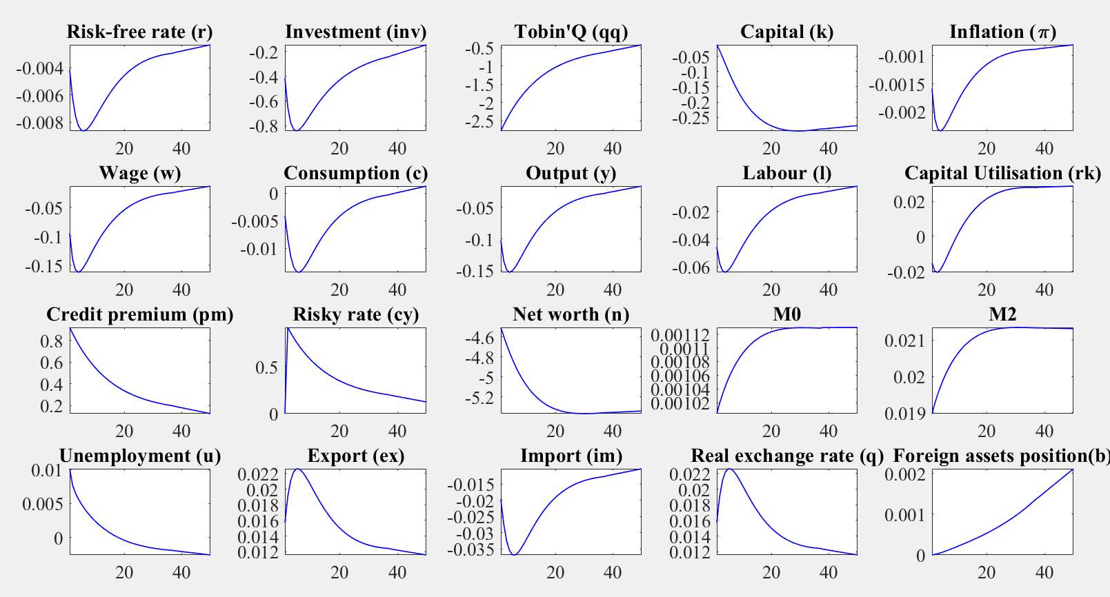
which gave me the plot as below:

I wanted to add the error band (1unit standard deviation) as :

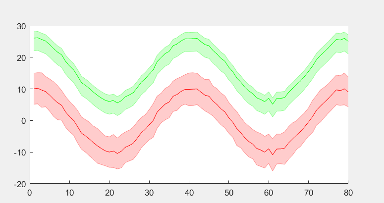
shadedErrorBar.m (5.1 KB) demo_shadedErrorBar.m (1.9 KB)
IRFfull.csv (11.6 KB)

The shaded error bar M files are attached…

Where does the uncertainty come from? Your IRFs seem to only include point estimates.

I used the model estimated parameters to generate these IRFs, but I didn’t do the estimation with Dynare, I am wondering if it is possible show the confidence bands on plots?
maybe there is no point investigating this at all.

Hi Julie,

A viable option is to create a time series of lower bounds and one of upper bounds of the desired confidence interval around the point estimates. You can then plot the point estimates with a solid line

hold on

and plot the two series with dashed lines in the same plot. You can do so for each variable.

To modify your code at the very minimum and roughly speaking, I mean something along the lines of, for instance,

clear all; close all; clc;
load IRFfull.csv; % Point estimates
load IRF_lower.csv % -1.96*st.dev
load IRF_upper.csv % +1.96*st.dev

varname=char('Risk-free rate (r)','Investment (inv)','Tobin''Q (qq) ',...
'Capital (k)','Inflation (\pi)','Wage (w)','Consumption (c)',...
'Output (y)','Labour (l)','Capital Utilisation (rk)',...
'Credit premium (pm)','Risky rate (cy)','Net worth (n)',...
'M0','M2','Unemployment (u)','Export (ex)','Import (im)',...
'Real exchange rate (q)','Foreign assets position(b)');

    for i=1:20
    subplot(4,5,i)  
    hold on
    plot(IRF_upper(:,i),'LineWidth',1,'b--');
    plot(IRFfull(:,i),'LineWidth',1,'r-');
    plot(IRF_lower(:,i),'LineWidth',1,'b--');
    axis tight;
    ax = gca;
    ax.YAxis.Exponent=0; 
    title(deblank(varname(i,:)));
    set(gca,'FontSize',16, 'FontName','Times');
    end

(I have not tested the code as I do not have your data at hand) :slightly_smiling_face:

thanks for your reply…

but how I am supposed to know the upper and lower bounds of the estimates…?

If you have the standard errors, you can compute the upper and lower bounds of the confidence interval. For example,

lower_bound_series=point_estimate-1.96*st.dev 
upper_bound_series=point_estimate+1.96*st.dev 

:slightly_smiling_face:

2 Likes

It depends on how you estimated the model/ the IRFs. Depending on your inference technique, there should be sampling variability or parameter uncertainty affecting the IRFs. Without knowing the estimation technique, it is impossible to tell.

1 Like

Hi, March
How I get the standard errors?
Thanks in advanced!

Wenddy

The comment I wrote before still applies: