It is possible to forecast shocks in dynare?
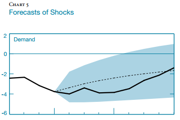
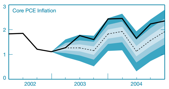
Notes: The dashed line represents the forecast of the relevant shock conditional on the posterior mean of the parameters while the solid line represents an estimate of the realization of the shock based on the Kalman smoother.
What is the definition of shocks here? By assumption, the innovations to a DSGE model are mean 0 and orthogonal to other information in the model. So they are not forecastable at all. What you can estimate is the value of the whole exogenous AR-process.
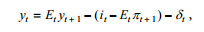
Thanks!! Demand shock here is the usual shock in the IS curve (in the paper). Thus, \delta_t.
This quote from the paper will clarify a little bit (sorry for the confusion).
“Chart 5 depicts the combinations of exogenous driving processes that, according to the estimated DSGE model, are responsible for the observed path of inflation, output, and the interest rate over the period we analyze. In each panel, the dashed line represents the evolution of the shock associated with the mean forecast while the solid line represents the sequence of shocks corresponding to the actual realization of the observable variables.”
It seems they take the estimated mean forecast as a restricted path, and then they call the structural shocks needed to match that path as “forecast of shocks”. Just speculating…
Lemme ask though, if my speculation above is the case and the mean forecasts are smooth (i.e., less variation), the structural shocks needed to match it will also be smooth, yeah?
I guess \delta_t follows an exogenous process with persistence. So they indeed seem to show the filtered values for \delta_t and compare them to the smoothed values.
Yes, indeed \delta_t (\delta_t, demand shock) follows an exogenous stochastic process in the paper.
Say, I have \delta_t = \rho \delta_{t-1} + \varepsilon^{\delta}_t…and I want to look at the importance of estimated demand shock in driving endogenous variables;
- I can fix \varepsilon^{\delta}_t to a constant using
simult_ command. Thus, examining the evolution of endogenous variables in the absence of demand shock.
- So like fixing \varepsilon^{\delta}_t to a constant (where \delta_t then exponentially falls over time with no short-run variations) \approx fixing \delta_t to a constant (i.e., a flat line over time with no short-run variations), right?
- Like in BCA, they fix \delta_t to a constant, but I guess fixing \varepsilon^{\delta}_t to a constant will equally suffice…
I would simply run a shock_decomposition.
Oh yeah, I see. The shock decomposition graph can also be used to study a given episode of the data. However, it seems it cannot tell you how endogenous variables will evolve in the presence or absence of a particular shock.
For example, it can tell you the contribution of preference shock to the inflation rate from, say, period 2000:1 to 2003:1, but not the direction of the inflation rate over that period in the presence of only a preference shock (and all other shocks being constant).
We have to pass the estimated smoothed shock(s) through the model to predict the path of endogenous variables for a given period of interest. Not sure we can see that from the shock_decomposition graph. Or we can?
It depends what you are trying to do. The shock_decomposition contributions decompose the model into contributions you would get when simulating the model with one shock at a time. If you suddenly want to shut off a particular innovation but still want the autoregressive component continue to decay to 0 you indeed have to run that simulation yourself.
Yes, exactly that. For example, in the figure below, The dashed line represents a counterfactual inflation rate conditional on the Kalman smoother estimates of all shocks except for one shock—say demand shock. Of course, allowing for all shocks to vary will recover the data. But one can shut some shock down to examine its importance over a given period (what I am trying to do).
But since we refer to δ_t (=ρδ_{t−1}+ε^δ_t) as a shock, shutting it down in my thought sort of means assuming δ_t = constant (thus, a flat line).
In dynare, however, we can only shut ε^δ_t down via simult_(), and hence δ_t will decay over time to zero (as you said)…with no fluctuations.
May I ask this:
Whether δ_t decays to zero (with no fluctuations) or it is just a flat line (with no fluctuations) seems not to matter much, right?. Thus, if we can normalize simulated paths and just look at short-run dynamics for a given period of the data that we care about.
The usual way is to indeed just shut off \varepsilon_t for t>t_0. Otherwise, there would be a discrete jump from the last value to 0.