Estimation problem onLog data density is Inf and modified harmonic mean estimator

Dear all,

I am new to estimation.

I’ve encountered the problem as the following:

The support of the weighting density function is not large enough…

Estimation::marginal density: I increase the variance of this distribution.

There’s probably a problem with the modified harmonic mean estimator.

And the result is shown below.

I don’t know what to look at, what the results mean, and how to adjust.

Could anyone help me with this?

I tried different mean and sd in the prior, all get the same problem.


hmdy521.mod (6.1 KB)
hm.mat (72.2 KB)
hm.m (2.0 KB)

hm.m is the file I generate the data.
hmdy521.mod is the estimation mod file.

Thanks a lot!

The f_qhncss is missing to run your file.

f_qhncss.m (1.2 KB)
sorry.

It seems your mode finding gets stuck as it cannot explain the data. Have you tried simulating data from your model and comparing it to the actual observables? It may be that there is a scaling issue.

Thanks a lot for the suggestion.

I just tried, the result is like the following. the red is my observable data, the blue is the simulated data.

Not sure it’s what you suggested, you can run the comparesvso.m file to generate the result.

comparesvso.m (593 Bytes)
hmdy521s.mod (6.3 KB)

comparesvso.m is the file compare the data.
hmdy521s.mod is the simulated mod file. it just deleted the estimation part compared to hmdy521.mod.

You can see an order of magnitude difference. It seems that you specify 1 percent as 1 in the data, but 0.01 in the model. That may explain part of the difference. In any case, for the given shock standard deviations, your model is unable to capture the data moments.

Oh, I see. Thanks!

I changed the stand error in the model to 1 to match the data. The comparison is now like the following:

I also tried correct this in the estimation file but the problem persists as in the following.

The updated file are the following:
comparesvso.m (593 Bytes)
hmdy521s.mod (6.2 KB)
hmdy521.mod (6.1 KB)

comparesvso.m is the file compare the data.
hmdy521s.mod is the simulated mod file.
hmdy521.mod is the estimation mod file.

You can see that your current model is incapable of simultaneously matching the various data series. Trying to estimate one parameter only will not change that.

I see. Will change the calibration of the model parameter help or will estimating more parameters help? How about add more shocks.

I tried another data, the marginal density seems been calculated, but the result seems still bad.

hmdy5211.mod (6.1 KB)

Yes, you should try to give the model a more plausible parameterization before estimating some of the parameters.

Thanks a lot!

May I know which aspect I should look at when comparing the simulated data and my observed data? is it only the magnitude(variance)? Is there any other thing I need to pay attention to?

I’m also curious that, In estimation, what does it mean to have 1 shock vs 2 shocks make difference to the result (posterior mean and posterior distribution)

Will more shocks help produce better empirical moments?

May I double-check with you the following:

I’ve read other posts and just notice that I’ve used method 1 (in the post below) to compare the simulated and observable data. But you said it’s wrong because the estimation code doesn’t work, I think I don’t have the estimated data to bring back to the model to do stoch_simul. So, is what I did still correct? And can I still use stoch_simul after the estimation block even when the estimation code doesn’t work?

Another question:

I am also not very familiar with what’s simulated data. e.g. if there is only 1 shock in the model, periods=1000, is the simulated data the irf of the endogenous variables (e.g. y) at the first period (y1), after drawing a value from the exogenous shock process, and then average the first-period value, y1 across the no of draws. Definitely wrong. I just don’t know how the simulated data is varied across time and how’s it averaged across what random process.

So, does it mean there is a shock drawn every period to simulate the data? e.g. if periods = 1000, at period 1, a shock is drawn, and at period 2, a shock is drawn?

So, what are these 1000 shocks doing in the policy function, is it averaged to be treated as the initial shock, or is it given a shock every period one by one to 40 periods, then what is the value of y, is it the irf of y at the first period after the shock?

Thank you.

  1. The goal of full information estimation is to find parameters to fully explain the data. That is “easier” if there are more parameters to vary. Estimation is particularly problematic if your shock standard deviations are unsuitable to allow for shocks big or small enough on average to explain the data realizations. That’s why having more estimated shocks often makes estimation easier, because it allows for more degrees of freedom when fitting the data.
  2. What I was suggesting is: put in likely parameter values (starting values for estimation) and simulate your data for the observables from the model using stoch_simul. If the variance of the simulated data is orders of magnitude different than the observed data, you still have a problem.
  3. If you put periods>0, Dynare will simulate data from the model by drawing random shocks for each period and iterating the policy functions forward in time. This is different from IRFS where you are asking about the effect of a one-time shock at period 0 (or the more complicated GIRFs at higher order).

I understand now. Thanks a lot for the explanation!

For 3. I am still a bit confused about the simulation process. May I have an example.
For my understanding:
e.g. for the TFP shock e (logA=rho*logA(-1)+e) with Normal distribution N(0,1), to get the simulation series for output y in simple RBC model, in period 1, there is a TFP shock of value e.g. e=0, I denote ‘time’ as the response/reaction period of this shock , i.e. e(period, time)= e(1,1)= 0, A(1,1)=1 (for future reaction of A under this shock, logA(1,2)= rho*logA(1,1)), y(1,1) have some value. In period 2, there is a new shock drawn of value e.g. e=1, then
e(period, time)= e(2,1)= 1, A(2,1)=e
(for future reaction of A under this shock, logA(2,2)= rho*logA(1,1)=rho), y(2,1) have some other value, …, so the simulation series for y, is the y(1,1), y (2,1), y(3,1), y (4,1), y(5,1), y (6,1).
Is this correct?

Thank you!

Dear Professor,

After reading your paper (from “A Guide to Specifying Observation Equations for the
Estimation of DSGE Models” ):

I found my parameter value block contains fsolve function, so that the steady state (ss) of two variables (those ss are used in the model block) are given by fsolve and is also determined by some other parameters, I’m afraid when doing the estimation, if I estimate the parameter in fsolve function, my ss in the parameter value block won’t update, and I cannot put fsolve in the model block
as well, I think which may cause some problem, may I know how can I avoid the dependence problem.

is there any way I can put fsolve in the model block, or how can I avoid this problem.

Thanks a lot!

function:
f_qhncss.m (1.2 KB)

mod file:hmdy522.mod (6.3 KB)

  1. Yes, this description of the simulation is correct.
  2. You should move the parameter setting part to a steady_state_model-block. See e.g. example3.mod of Dynare’s example folder
    or at: examples · master · Dynare / dynare · GitLab

Thanks a lot for the reply.

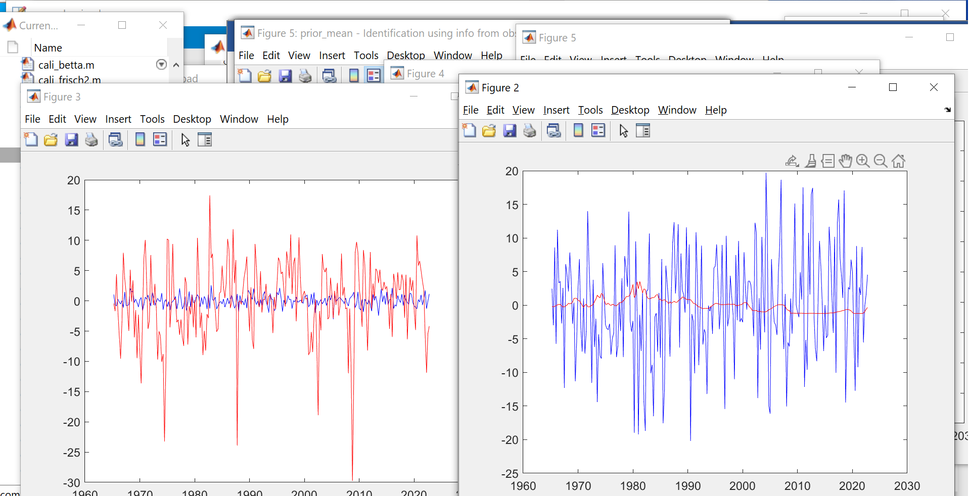
  1. Just want to double check with you, that the simulation data of the model is the separate different first-period irf of iid shocks combined together.
    If this is the case, I am just curious, why compare the detrended empirical data with the irf of the first period, why not the first 5 or 10, or the second. Is there any autocorrelation considered in the simulation data from model. May I know if there is any theory backing this simulation or comparison.

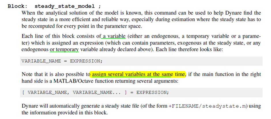
  2. I have some problem using fsolve in the steady_state_model block.
    I read this in the dynare manual:


    It says I can assign several variables at the same time, but I am not sure how to write it, have problem doing this.
    My code is the following:

steady_state_model;

[Qh,Nc] = ss2var(alfa,delttass,Ass,rss,gss,hb,deltah,ksi,epsilonass,Qh0,Nc0);

end;

ss2var is the steady state calculation function as the following:

function XX_ss=ss2var(alfa,delttass,Ass,rss,gss,hb,deltah,ksi,epsilonass,Qh0, Nc0)
options=optimset(‘Display’,‘Final’,‘TolX’,1e-10,‘TolFun’,1e-10);
[XX_ss,fval,exitf] = fsolve(@(XX)f_qhncsp(XX,alfa,delttass,Ass,rss,gss,hb,deltah,ksi,epsilonass),[Qh0 Nc0]);

f_qhncsp will return the value of Qh and Nc as:

function diff=f_qhncsp(XX,alfa,delttass,Ass,rss,gss,hb,deltah,ksi,epsilonass)

Qh = XX(1);
Nc = XX(2);


diff(1) = delttass/(1-N)-W/Ct;
diff(2) = QhH - gamCt/(1-(1-deltah)/R);

it returns:

Processing outputs …
done
Preprocessing completed.

Error using ss2var
Too many output arguments.

Error in hm72fsdraft.steadystate (line 15)
[ys_(8),ys_(13)]=ss2var(params(1),params(2),params(3),params(4),params(5),params(6),params(7),params(8),params(9),params(43),params(44));

Error in evaluate_steady_state_file (line 53)
[ys,params1,check] = h_steadystate(ys_init, exo_ss, params);

Error in evaluate_steady_state (line 254)
[ys,params,info] = evaluate_steady_state_file(ys_init,exo_ss,M, options,steadystate_check_flag);

Error in resid (line 66)
evaluate_steady_state(oo_.steady_state,M_,options_,oo_,0);

Error in hm72fsdraft.driver (line 789)
resid;

Error in dynare (line 281)
evalin(‘base’,[fname ‘.driver’]);

Thanks a lot.
hm72fsdraft.mod (8.3 KB)
ss2var.m (263 Bytes)
f_qhncsp.m (1.3 KB)

And when I try to solve the above problem of sereval variables.

my mod file has run into a loop in fslove,

could you please help me on this.

Thanks a lot.
Qh_ss_helper.m (277 Bytes)
Nc_ss_helper.m (278 Bytes)
hm72fsdrafts.mod (8.3 KB)

Sorry, it is actually working. I just need to wait a bit longer so that it can produce the result.