Hi.
I do not understand how to use a sequence of mode_compute. I started to estimate my model using first a mode_compute=6 but my mode check plots and convergence graphs are not so good. For this case, I read that it is a good thing to estimate the model again with a new mode_compute.
- Do I have to load first with mode_compute=0 and then use again a estimation command with a mode_compute=7 (for example) or should I put mode_compute=7 together with mode_file?
That is something like:
estimation(order=1,datafile=‘mymodel_data.xlsx’,mode_file=mymodel_mode, mode_compute=0,mode_check);
estimation(order=1,datafile=‘mymodel_data.xlsx’, mode_compute=7,mode_check);
or
estimation(order=1,datafile=‘mymodel_data.xlsx’,mode_file=mymodel_mode, mode_compute=7,mode_check);
- I tried to use the last one and I get:
The mode_file option of the estimation st
The mode_file option of the estimation statement is incompatible with the use_calibration option
If I suppress the estimated_params_init block, it runs, although I am not sure what it is happening. Does it mean that the estimation uses the mean (or mode) of the first posterior distribution as initial point?
- I usually have success only with mode_compute=6. Is there any benefit in using a sequence with mode_compute=6 twice or will it be prone to be stucked in the same results?
Thank you.
Thank you, professor Pfeifer. Your comments were very helpful.
I managed to get some good mode plot but the MCMC univariate/multivariate convergence plots are still bad.
- Do you have any suggestion to improve them?
- Are they suppose to be stabilized horizontally and close to each other only at the end of the plot or in the entire plot?
Could you provide trace plots?
Here they are.
I did not know about these graphs and I am not sure that I understood this intuition.
generate_trace_plots(1).zip (1.0 MB)
Thanks, professor Pfeifer. I read Pfeifer (2014): “An Introduction to Graphs in Dynare” but I am not sure I understood everything. I would appreciate very much some comments about these questions:
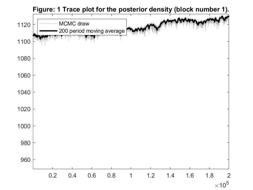
1 - The Figure 1 is a trace plot for the joint posterior density?
2 - Do I have to look at each parameter figures to verify if I have to change the burn-in sample? For example, in Figure 14 below, the initial draws of psi_pi are different from the last ones. Actually, the parameter draws seem to be stabilized only in the draws180.000-200.000. I think that I have to dismiss the draws that are very dependent of initial value, but I do not have to do it too much because it would cause a very concentrated posterior.
Looking at this graph, for me it is not clear where I should define the burn-in period. And other parameters may have other pattern, so what to do in this case?
3 - About your comment to “start mode-finding based on the last draw of the chain”, do you mean to use the mode_file and/or load_mh_file? I do not understand what are the differences between these commands.
Dear prof. Pfeifer, thank you very much for all the information.
I ran the model again and even with much more draws, it seems it is not converging (considering trace plot for posterior). I wonder if it is slow to converge because I am using just mode_compute=6.
I read in other posts that if the others mode_compute show problems with Hessian maybe a consequence of identification problem.
-
Do you think it is indeed a identification problem? If so, do you have any suggestions to solve it? The identification analysis seems to be ok, but identification strenght plot shows that some parameters have 0 strenght (relative to prior std). In addition, how can I reproduce this graph, since the parameters name are not readable because of this size?
-
For me, the graphs with prior and posterior seem to be strange. Sometimes the mode are very far from posterior. Is it acceptable or a consequence of some other problem?
-
Some mode check plot seem to be defined in a very small range (axis X). Due to previous results I assume that these parameters have good mode check plots, however I do not understand why they have the small range.
Files.zip|attachment (399.3 KB)
Thank you
The psi_pi and psi_pi_star with their uniform distributions run into the prior bounds. When using a normal distribution for them things looks a lot better. Also try mode_compute=5. It results in a significant improvement in the mode.
Thank you again, prof Pfeifer.
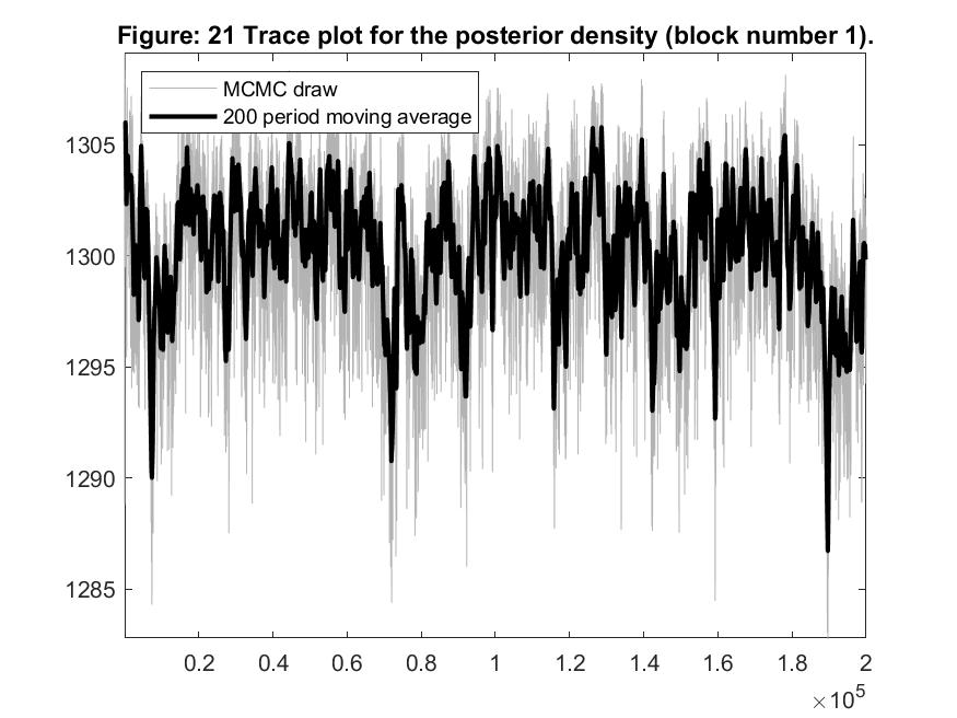
With your comments, I ran the model (changing the priors and mode_compute=5) and it seems it converged:
The other results bring me some more questions:
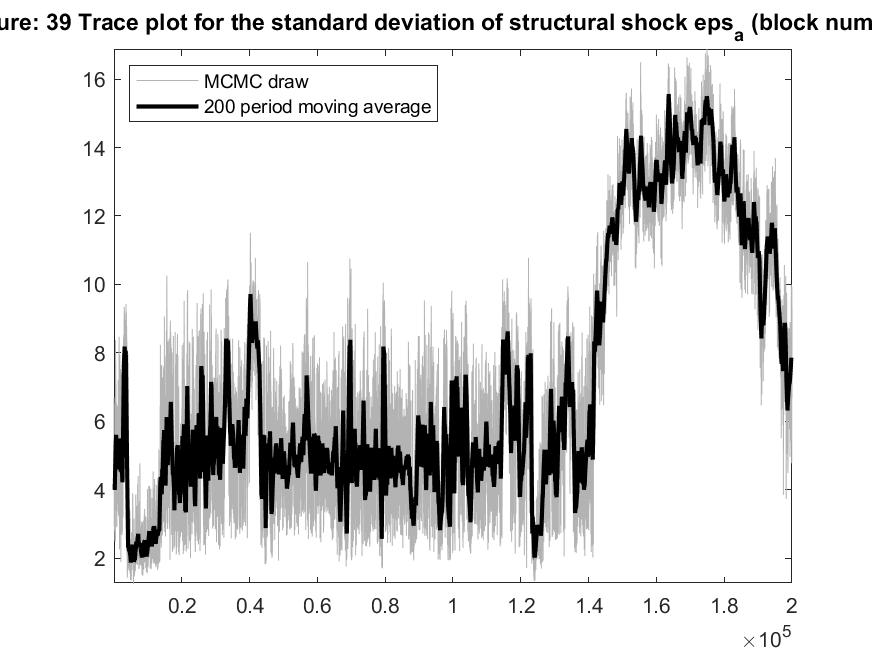
- Some parameters trace plots are not good, specially for std of eps_a. The same happens for univariate diagnostics plot. Should I be worried? For example, do I have to use specific parameter scale?
- In Mode check and estimation marginal density I received a message:
Warning: Matrix is close to singular or badly scaled. Results may be inaccurate
And in mode check I received also the messages (only for these 3 values):
mode_check:: could not solve model for parameter psi_pistar at value 0.775, error code: 4
mode_check:: could not solve model for parameter psi_pistar at value 0.853, error code: 4
mode_check:: could not solve model for parameter psi_pistar at value 0.930, error code: 4
Is there a problem?
- The identification analysis seems to be ok, but identification strenght plot shows that some parameters have 0 strenght (relative to prior std). Why does it happen?
Thank you for your comments, professor Pfeifer. They were very clear and helpful.