Hi!
I have a model, which produces IRFs, time paths and variance decomposition, but which gives me the following error message:
Blockquote
EIGENVALUES:
Modulus Real Imaginary
      0.1329           0.1329                0
      0.2837           0.2837                0
         0.5              0.5                0
         0.5              0.5                0
         0.5              0.5                0
         0.5              0.5                0
         0.5              0.5                0
         0.5              0.5                0
         0.5              0.5                0
         0.5              0.5                0
         0.5              0.5                0
      0.6672           0.6653          0.04953
      0.6672           0.6653         -0.04953
      0.8386           0.7033           0.4568
      0.8386           0.7033          -0.4568
      0.9985           0.9985                0
       1.039            1.039                0
       1.493            1.452           0.3488
       1.493            1.452          -0.3488
       1.808            1.732           0.5188
       1.808            1.732          -0.5188
       3.585            3.585                0
  1.262e+016       1.262e+016                0
   1.06e+017        1.06e+017                0
         Inf             -Inf                0
There are 9 eigenvalue(s) larger than 1 in modulus
for 9 forward-looking variable(s)
The rank condition is verified.
What do I have to do now?
What is the error message? I do not see it.
Best,
Stéphane.
The two values in the last row are Inf and -Inf. This leads to problems in my model. How can I avoid values that become infinity.
No, this is not a problem. The generalized eigenvalues of the generalized Schur decomposition do not need to be finite. They are counted as unstable eigenvalues, and the reduced form solution is built by eliminating these eigenvalues (finite or not).
Best,
Stéphane.
You can find detailed explanations about this in the paper by Paul Klein (JEDC, 1999).
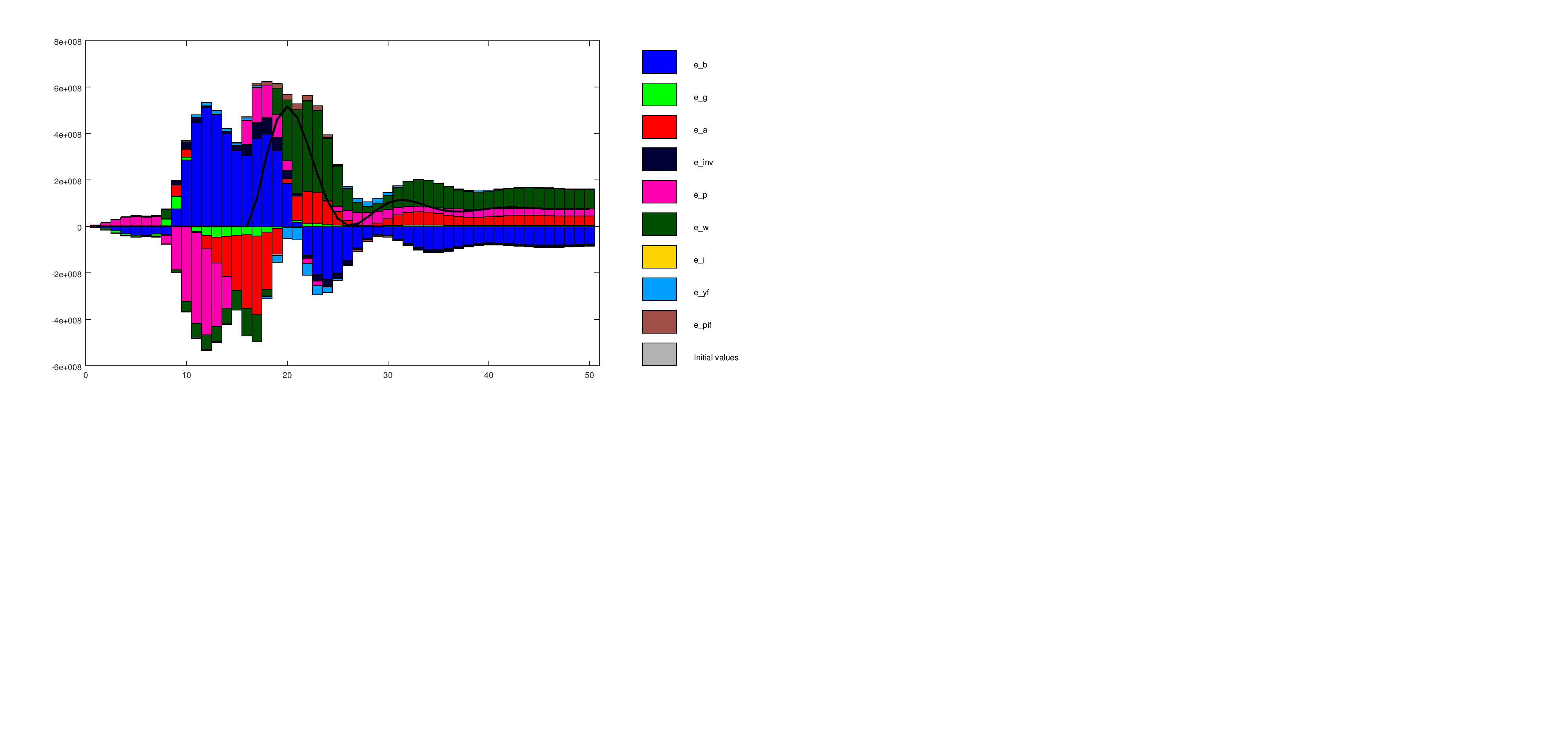
Thanks for your reply. But why do I get such strange graphs? I thought that this must be somehow related to numerical problems within the code, for example, because some values become infinity.
Your variable looks weird… It is zero at the beginning of the sample (maybe it is only a scaling issue here) and of order 10^8 after. What is this variable?
This is consumption. The problem is: My model has a steady state and the rank condition is verified, but the shock decomposition looks like this. So, I think there must be a numerical problem.
What is the steady state of consumption in your model? What is the mean of your consumption data? I still have doubts about the data you are using here.
Best,
Stéphane.
The steady state of consumption is 0.828231. I only use simulated data, ie. I simulate the model for 50 periods, save the data and then use these simulated variables to conduct the historical shock decomposition. Maybe some steady state values cause the problems, because they are extremely small, but not exactly zero. However, I do not understand why this occurs, for example, for ei, which is the monetary policy shock, defined as AR(1) process with autocorrelation 0.5 and stderr 1, while the other shocks have a different steady state.
Here is the full list of my steady state results
c                                0.828231
invest                           0.891056
q                                0
ks                               0.891056
u                                -4.61298e-016
k                                0.891056
mup                              -0.604266
pih                              0.749343
pi                               0.749343
r                                5.55112e-016
muw                              -0.0317585
w                                0.863237
l                                0.0278185
yh                               0.4038
y                                0.0367216
i                                0.749343
eb                               0
eg                               0
ea                               0
einv                             0
ep                               0
ew                               0
ei                               -8.32667e-017
yf                               0.0249781
pif                              0.749343
eyf                              0
epif                             0
qq                               1.65787e-018
The simulated path for consumption is very far from the steady state. Did you simulate the data with a second order approximation? This may explain the huge gap between the simulated data and the steady state. You should simulate the data with order=1 option in stock_simul command (or use the pruning option).
Best,
Stéphane.
That said, looking at the number, I find your steady state very strange. If y, invest and c are output, investment and consumption, I don’t understand the meaning of such a steady state (output is very small compared to consumption plus investment).
Thanks for the reply, but I still get the same results. Below are the simulated moments for consumption. The variance is extremely large.
     VARIABLE              MEAN       STD. DEV.        VARIANCE        SKEWNESS        KURTOSIS
c      6.139269       23.306375      543.187102        1.678707        2.509157                 2.509157
Output is defined as difference between demand (according to the goods market equilibrium) and supply (according to the factors from the production function). This might lead to a small output compared to consumption. However, this approach works fine in a lot of models, that I have used in the past.
Please provide the files and explain how exactly you generated the simulated data
The mean does not look consistent with the numbers in the plot… Which seem always positive and of order 10^8.
I do not understand your answer regarding the steady state, how output can be more than one hundred times smaller than the sum of consumption and investment (maybe I am looking at the wrong numbers).
Here is the mod-file, which also contains the procedure to simulate, save and use the simulated data:
model1.mod (3.2 KB)
Output is yh 0.4038, but it is true that it is small, it’s only a quarter of the sum of consumption and investment. Output y is the output of the currency union, weighted by the country size, which is 0.031.
@pnovak Please do not cross-post the same issue twice. Your model still has at least two mistakes. See my reply at Small open economy in a currency union