When I run the model, it indicates that there is 3 colinear relationships between the variables and the equations,but I can not find the problem,although much time have been spent on it. Thanks for your help for all.
In my model ,it contains four sectors : family ,entrepreneur,commercial bank and central bank,the trouble may happens in commercial bank,but the concrete problem can not be found and do not know how to modify the model to solve the problem.
This is my model:
close all;
var L C W K I Y Rk Rd Re e A vp pihash pi mc x1 x2 Rl tau D N ;
predetermined_variables K;
varexo ea eRe etau;
parameters psil psie eta beta delta v gamma zetap mu psim rhoa rhoRe rhotau sigmaa sigmaRe sigmatau psipi psiy;
parameters Ls Cs Ws Ks Is Ys Rks Rds Res es As vps pihashs pis mcs x1s x2s Rls taus Ds Ns ;
psil=1;
psie=1;
eta=1.44018;
beta=0.99;
delta=0.012;
v=2;
gamma=0.4;
zetap=0.75;
mu=2;
psim=0;
rhoa=0.9;
sigmaa=0.1;
rhoRe=1;
sigmaRe=0.1;
rhotau=1;
sigmatau=0.1;
psipi=1;
psiy=1;
%steady state calculation
pis=1;
taus=0.1;
As=1;
Ls=0.64;
Rds=pis/beta;
Res=Rds;
Rks=(1/beta)-(1-delta);
Rls=((1+Rds)/(1-taus))-1;
pihashs=((pis^(1-mu)-zetap)/(1-zetap))^(1/(1-mu));
vps=(1-zetap)*(pis/pihashs)^mu/(1-pis^mu*zetap);
mcs=((1-zetap*beta*pis^mu)/(1-zetap*beta*pis^(mu-1)))*(pihashs/pis)*((mu-1)/mu);
gs=(mcs*gamma/(Rks*(1+psim*Rls)))^(1/(1-gamma));
Ks=gs*Ls;
Is=delta*Ks;
Ws=mcs*(1-gamma)*Ks^gamma*Ls^(-gamma)/(1+psim*Rls);
Ys=(As*(Ks^gamma)*(Ls^(1-gamma)))/vps;
Cs=Ys-Is;
es=((Rds-Res)/(Cs*psie*Rds))^(1/(-v));
x1s=mcs*Ys/(Cs*(1-zetap*beta*pis^mu));
x2s=Ys/(Cs*(1-zetap*beta*pis^(mu-1)));
Ds=(Ws*Ls+Rks*Ks)*(1+psim*Rls);
Ns=((1-taus+Rds)/(1+Rls))*Ds;
model;
%(1) labor supply
psil*exp(eta*L)=exp(W)/exp(C);
%(2) deposit
1/exp(C)=beta*(1/exp(C(+1)))*exp(Rd)/exp(pi(+1));
%(3) home Euler equation
1/exp(C)=beta*(1/exp(C(+1)))*(exp(Rk(+1))+1-delta);
%(4) decp
psie*exp((-v)*e)=(1/exp(C))*(exp(Rd)-exp(Re))/exp(Rd);
%(56) No arbitrary
exp(Rk)+1-delta=exp(Rd);
exp(Rd)=exp(Re);
%(7) resource constraint
exp(Y)=exp(C)+exp(I);
%(8) capital accumulation
exp(K(+1))=exp(I)+exp(K)*(1-delta);
%(9) wage
exp(W)=(1-gamma)*exp(mc)*exp(A)*exp(gamma*K)*exp(-gamma*L)/(1+psim*Rl);
%(10) capital returns
exp(Rk)=gamma*exp(mc)*exp(A)*exp((gamma-1)*K)*exp((1-gamma)*L)/(1+psim*Rl);
%(11) the sticky price equation
exp(pihash)=(mu/(mu-1))*exp(pi)*(exp(x1)/exp(x2));
%(12) the production technology
exp(Y)=exp(A)*exp(gamma*K)*exp((1-gamma)*L)/exp(vp);
%(13) the price dispersion
exp(vp)=(1-zetap)*exp(-mu*pihash)*exp(mu*pi)+exp(mu*pi)*zetap*exp(vp(-1));
%(14) inflation evolution
exp((1-mu)*pi)=(1-zetap)*exp((1-mu)*pihash)+zetap;
%(15) the auxiliary x1
exp(x1)=(1/exp(C))*exp(Y)*exp(mc)+zetap*beta*exp(mu*pi(+1))*exp(x1(+1));
%(16) the auxiliary x2
exp(x2)=(1/exp(C))*exp(Y)+zetap*beta*exp((mu-1)*pi(+1))*exp(x2(+1));
%(17) bank
exp(D)*(1-exp(tau)+exp(Rd))=exp(N)*(1+exp(Rl));
%(18) bank equilibrium
1+exp(Rl)=(1+exp(Rd))/(1-exp(tau));
%(19) technology shock
A=rhoa*A(-1)+ea;
%(20) reserve shock
tau=rhotau*tau(-1)+etau;
%(21) decp rule
(Re/Res)=rhoRe*Re(-1)/Res+(1-rhoRe)*(psipi*(pi/pis)+psiy*(Y/Ys))+eRe;
end;
initval;
L=log(Ls);
C=log(Cs);
W=log(Ws);
K=log(Ks);
I=log(Is);
Y=log(Ys);
Rk=log(Rks);
Rd=log(Rds);
Re=log(Res);
e=log(es);
A=log(As);
vp=log(vps);
pihash=log(pihashs);
pi=log(pis);
mc=log(mcs);
x1=log(x1s);
x2=log(x2s);
Rl=log(Rls);
tau=log(taus);
D=log(Ds);
N=log(Ns);
end;
shocks;
var ea=.01^2;
var etau=.01^2;
var eRe=.01^2;
end;
resid(1);
steady;
check;
model_diagnostics;
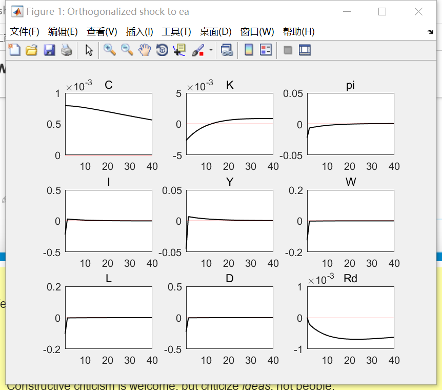
stoch_simul(order=1) Y C I W L K pi D Rd;
These are my results and problems:
dynare D
Starting Dynare (version 5.0).
Calling Dynare with arguments: none
Starting preprocessing of the model file ...
Found 21 equation(s).
Evaluating expressions...done
Computing static model derivatives (order 1).
Computing dynamic model derivatives (order 1).
Processing outputs ...
done
Preprocessing completed.


Residuals of the static equations:

Equation number 1 : -7.691e-07 : 1
Equation number 2 : 0 : 2
Equation number 3 : 0 : 3
Equation number 4 : 0 : 4
Equation number 5 : 0 : 5
Equation number 6 : 0 : 6
Equation number 7 : 0 : 7
Equation number 8 : 0 : 8
Equation number 9 : 0 : 9
Equation number 10 : 0 : 10
Equation number 11 : 0 : 11
Equation number 12 : 0 : 12
Equation number 13 : 0 : 13
Equation number 14 : 0 : 14
Equation number 15 : 0 : 15
Equation number 16 : 0 : 16
Equation number 17 : 0 : 17
Equation number 18 : 0 : 18
Equation number 19 : 0 : A
Equation number 20 : 0 : tau
Equation number 21 : 0 : 21


STEADY-STATE RESULTS:

L      		 -0.446287
C      		 0.907222
W      		 0.26449
K      		 3.22487
I      		 -1.19798
Y      		 1.02218
Rk     		 -3.81213
Rd     		 0.0100503
Re     		 0.0100503
e      		 Inf
A      		 0
vp     		 0
pihash 		 0
pi     		 0
mc     		 -0.693147
x1     		 0.778542
x2     		 1.47169
Rl     		 0.209812
tau    		 -2.30259
D      		 0.329028
N      		 0.172639

EIGENVALUES:
         Modulus             Real        Imaginary

            0.75             0.75                0
             0.9              0.9                0
          0.9361           0.9361                0
               1                1                0
               1                1                0
           1.122            1.122                0
           1.238            1.238                0
           1.277           -1.277                0
           1.347            1.347                0
       7.175e+43       -7.175e+43                0


There are 5 eigenvalue(s) larger than 1 in modulus
for 5 forward-looking variable(s)

The rank condition is verified.

MODEL_DIAGNOSTICS:  The Jacobian of the static model is singular
MODEL_DIAGNOSTICS:  there is 3 colinear relationships between the variables and the equations
Relation 1
Colinear variables:
e
Rl
tau
D
N
Relation 2
Colinear variables:
e
Rl
tau
D
N
Relation 3
Colinear variables:
e
Rl
tau
D
N
Relation 1
Colinear equations
     4     6
Relation 2
Colinear equations
    21
Relation 3
Colinear equations
    20
MODEL_DIAGNOSTICS:  The singularity seems to be (partly) caused by the presence of a unit root
MODEL_DIAGNOSTICS:  as the absolute value of one eigenvalue is in the range of +-1e-6 to 1.
MODEL_DIAGNOSTICS:  If the model is actually supposed to feature unit root behavior, such a warning is expected,
MODEL_DIAGNOSTICS:  but you should nevertheless check whether there is an additional singularity problem.
MODEL_DIAGNOSTICS:  The presence of a singularity problem typically indicates that there is one
MODEL_DIAGNOSTICS:  redundant equation entered in the model block, while another non-redundant equation
MODEL_DIAGNOSTICS:  is missing. The problem often derives from Walras Law.
> In dyn_first_order_solver (line 277)
  In stochastic_solvers (line 251)
  In resol (line 119)
  In stoch_simul (line 109)
  In D.driver (line 482)
  In dynare (line 281)
警告: 矩阵为奇异工作精度。
> In dyn_first_order_solver (line 297)
  In stochastic_solvers (line 251)
  In resol (line 119)
  In stoch_simul (line 109)
  In D.driver (line 482)
  In dynare (line 281)
警告: 矩阵为奇异工作精度。

MODEL SUMMARY

  Number of variables:         21
  Number of stochastic shocks: 3
  Number of state variables:   5
  Number of jumpers:           5
  Number of static variables:  11


MATRIX OF COVARIANCE OF EXOGENOUS SHOCKS
Variables          ea       eRe      etau
ea           0.000100  0.000000  0.000000
eRe          0.000000  0.000100  0.000000
etau         0.000000  0.000000  0.000100

POLICY AND TRANSITION FUNCTIONS
                                   Y               C               I               W               L               K              pi               D              Rd
Constant                    1.022176        0.907222       -1.197979        0.264490       -0.446287        3.224870               0        0.329028        0.010050
K(-1)                              0        0.861421               0               0               0        0.936084        0.192798            -Inf               0
Re(-1)                             0       32.129045               0               0               0       -3.984791       15.120630            -Inf               0
A(-1)                              0        0.253816               0               0               0        0.082316       -0.205069             Inf               0
vp(-1)                             0       -0.224406               0               0               0       -0.051926       -0.032407             Inf               0
tau(-1)                            0               0               0               0               0               0               0            -Inf               0
ea                                 0        0.078974               0               0               0       -0.157760       -0.91720817520278286072495862254468595712.000000               0
eRe                                0       47.320247               0               0               0       14.222771       65.747208-1282818264881313154549164093210624.000000               0
etau                               0               0               0               0               0               0               0-23854034316172736.000000               0

All endogenous are constant or non stationary, not displaying correlations and auto-correlations

Total computing time : 0h00m01s
Note: warning(s) encountered in MATLAB/Octave code