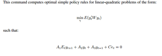
Because we are choosing \gamma (a constant) to minimize our objective (here, the objective of the central bank), commitment or discretionary does not matter, right?
AFAIK, an OSR is always a commitment rule.
Like the central bank chooses \gamma at period 0 for all t, and commits to it? If I may ask, how would that be different from choosing \gamma sequentially for each t?
Or osr is always a commitment rule because even if the CB chooses \gamma sequentially, it does not change from period to period, right? Thanks!
Yes, it’s commitment because the central bank uses a rule with a fixed parameter and does not reoptimize. Say there is government debt, which is predetermined. The government may have a temptation in the first period to inflate it away and then implement a stable, low inflation rate. We prevent the central bank from doing that here, because it is committed to the same rule in all periods.
Dear Professor,
I have another question regarding discretionary policy. I have a question regarding how to plot a “Taylor frontier” in the case of a discretionary monetary policy. Usually, I see the Taylor frontier constructed by varying the coefficients in a Taylor rule (under commitment) and then plotting the resulting trade-off between inflation and output variance.
However, if the central bank re-optimizes each period under discretion, it seems that the policy might not be representable by a fixed-coefficient Taylor rule. Instead, is the optimal reaction(Taylor rule) coefficients time-varying? Is the weight(lambda) in welfare \pai^2+\lambda y^2 time varying? I’m really confused, because it seems the lambda is fixed by parameter combination in your Gali ch5 code.
Is it still possible to draw a similar frontier under a truly discretionary setup?
Thank you very much for your time. Sorry if it’s fundamental but I 'm quite confused.
I am not sure I understand the question. The type of efficiency frontier you describe is about varying weights in an optimal simple rule chosen by the user. That does not make sense in the context of Ramsey or discretionary policy where the policy is unique (but generally cannot be represented as a rule).
A different type of efficiency frontier involves varying the weight on inflation or output in the objective function. That can generally be done with discretionary policy. But in many contexts, there is a unique weighting given by the utility function of the agents. That is for example the case in Gali’s model.
discre.mod (2.8 KB)
Dear Professor,
I attached your Gali Ch5 discretionary mod and your policy frontier code. Policy frontier - Optimal Policy - Dynare ForumBur it got errors.
error stochastic_solvers (row 210 )
b(:,cols_b) = jacobia_(:,cols_j);
^^^^^^^^^^^
error resol (row 115 )
[dr, info] = stochastic_solvers(dr, check_flag, M_, options_, exo_steady_state, exo_det_steady_state);
^^^^^^^^^^^^^^^^^^^^^^^^^^^^^^^^^^^^^^^^^^^^^^^^^^^^^^^^^^^^^^^^^^^^^^^^^^^^^^^^^^^^^^^^
Error osr.objective (row 46 )
[oo_.dr,info,M_.params] = resol(0,M_,options_,oo_.dr ,oo_.steady_state, oo_.exo_steady_state, oo_.exo_det_steady_state);
^^^^^^^^^^^^^^^^^^^^^^^^^^^^^^^^^^^^^^^^^^^^^^^^^^^^^^^^^^^^^^^^^^^^^^^^^^^^^^^^^^^^^^^^^^^^^
Error osr.run (row 115 )
[loss,info]=osr.objective(par_0,M_,oo_,options_,i_params,inv_order_var(i_var),W(i_var,i_var));
^^^^^^^^^^^^^^^^^^^^^^^^^^^^^^^^^^^^^^^^^^^^^^^^^^^^^^^^^^^^^^^^^^^^^^^^^^^^^^^^^
Error discre.driver (row 359 )
[info, oo_, options_, M_] = osr.run(M_, options_, oo_, {}, M_.osr.param_names, M_.osr.variable_indices,M_.osr.variable_weights);
^^^^^^^^^^^^^^^^^^^^^^^^^^^^^^^^^^^^^^^^^^^^^^^^^^^^^^^^^^^^^^^^^^^^^^^^^^^^^^^^^^^^^^^^^^^^^^^^^^^
Error dynare (row 308 )
evalin(‘base’,[fname ‘.driver’]);
^^^^^^^^^^^^^^^^^^^^^^^^^^^^^^^^
My question is this.Can discretionary and the policy frontier combine? I’m quite confused. Thanks professor for your time.Sorry I changed a lot of times,because I have in a class.
Without the code it is impossible to tell. But I still don’t understand what you are trying to do. You did not even clearly define what you mean with “policy frontier”.
close all
%----------------------------------------------------------------------------------------------------------------
var pi y_gap y_nat y r_e y_e x r_nat r_real i n m_growth_ann a u r_real_ann i_ann r_nat_ann
pi_ann p;
varexo eps_u eps_a;
parameters alpha beta sigma theta epsilon phi eta rho_u rho_a psi omega lambda gamma kappa w_pi;
%----------------------------------------------------------------------------------------------------------------
%
alpha=1/2;
beta=0.985;
sigma=2;
theta=2/3;
epsilon=6;
phi=2;
eta=4;
rho_u=0.8;
rho_a=0;
w_pi=0.5;

%
psi=(1+phi)/(sigma*(1-alpha)+phi+alpha);

omega=(1-alpha)/(1-alpha+alpha*epsilon);
lambda=(1-theta)*(1-beta*theta)/theta*omega;
gamma=sigma+(phi+alpha)/(1-alpha);
kappa=gamma*lambda;

%----------------------------------------------------------------------------------------------------------------
model(linear);

x =-1/sigma*(i-pi(+1)-r_e)+x(+1);

pi=beta*pi(+1)+kappa*x+u;

r_e=sigma*(y_e(+1)-y_e);
y_e=psi*a;
y_gap=x+(y_e-y_nat);

y=a+(1-alpha)*n;

m_growth_ann=4*(y-y(-1)-eta*(i-i(-1))+pi);

r_nat=sigma*psi*(a(+1)-a);
y_nat=psi*a;
y_gap=y-y_nat;

r_real=i-pi(+1);

pi=p-p(-1);

u=rho_u*u(-1)+eps_u;
a=rho_a*a(-1)+eps_a;

i_ann=4*i;
r_real_ann=4*r_real;
r_nat_ann=4*r_nat;
pi_ann=4*pi;
end;
%----------------------------------------------------------------------------------------------------------------
shocks;
var eps_u=1;
end;
%----------------------------------------------------------------------------------------------------------------
planner_objective w_pi*(pi^2) + (1-w_pi)*(x^2);
discretionary_policy(instruments=(i),irf=20,planner_discount=beta,discretionary_tol=1e-12) x pi p u;

options_.nofunctions=1;
options_.nocorr=1;
options_.noprint=1;
options_.irf=0;
options_.silent_optimizer=1;

options_.osr.opt_algo=9;

x_pos=strmatch('x',M_.endo_names,'exact');
pi_pos=strmatch('pi',M_.endo_names,'exact');

x_pos_M_.endo_names=strmatch('x',M_.endo_names,'exact');
pi_pos_M_.endo_names=strmatch('pi',M_.endo_names,'exact');

weight_grid=0:0.05:1;
n_grid_points=length(weight_grid);
var_x=NaN(n_grid_points,1);
var_pi=NaN(n_grid_points,1);

for grid_iter=1:n_grid_points
    M_.osr.variable_weights(pi_pos,pi_pos)=weight_grid(grid_iter);
    M_.osr.variable_weights(x_pos,x_pos)=(1-weight_grid(grid_iter));
    [info, oo_, options_, M_] = osr.run(M_, options_, oo_, {}, M_.osr.param_names, M_.osr.variable_indices,M_.osr.variable_weights);
    if oo_.osr.error_indicator==0
        var_x(grid_iter)=oo_.var(x_pos_M_.endo_names,x_pos_M_.endo_names);
        var_pi(grid_iter)=oo_.var(pi_pos_M_.endo_names,pi_pos_M_.endo_names);
    end
end

figure
plot(sqrt(var_x),sqrt(var_pi))
xlabel('sd x')
ylabel('sd \pi')
title('MP frontier')
Dear professor I attach the code here. In the code, I am using the discretionary_policy function, but I noticed that the OSR (Optimal Simple Rule) method is typically associated with commitment policy, where future expectations are taken into account.
The issue is that, in a discretionary policy setting, the central bank re-optimizes every period without committing to future actions, and I’m not sure if it’s possible to compute the policy frontier in a similar way.
Here’s my main question:
- Is it possible to plot the policy frontier under discretionary police? If yes, how can I modify the existing code to do this?How can I use different w_pi weights in the discretionary policy model to compute the variances of inflation and output gap, and plot the resulting policy frontier?
- Am I correct in understanding the differences between the calculations under discretionary and commitment policies in this context?
Thank you very much for your time !
Please again read my above post at Does dynare osr assumes committment or discretionary? - #6 by jpfeifer
and then answer what exactly you are trying to vary when plotting such a frontier. There are no weights that you could alter in fully optimal policies, which is different from the OSR case .
Thank you very much, professor. Let me confirm whether I fully understand your points correctly:
1.In micro-founded models like Galí, the central bank’s loss function is typically derived from the representative household’s welfare. Therefore, the relative weights on inflation and the output gap in such welfare-based objectives are determined endogenously and uniquely by deep structural parameters (such as preferences, price rigidities, and production technologies). Thus, these weights are fixed once the underlying parameters are chosen, and we cannot vary these weights to plot a policy frontier.
-
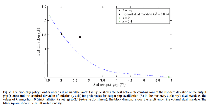
By contrast, in the case of an exogenously specified mandate-based central bank objective (such as this kinds of figure
from Optimal simple objectives for monetary policy when banks matter - ScienceDirect), the policymaker’s loss function weights are chosen arbitrarily. Thus, by varying these exogenous weights (e.g., the weight on output gap stabilization), we can indeed plot the resulting policy frontier. -
Therefore, whether we can plot a policy frontier by varying weights depends crucially on whether the central bank’s objective is welfare-based (endogenous and fixed weights) or mandate-based (exogenous and adjustable weights).
Additionally, OSR always assume exogenous, adjustable policy weights, hence allowing the frontier to be drawn easily. OSR does not differentiate explicitly between discretion and commitment, as it directly optimizes parameters of simple rules.
Ramsey and discretionary policies, when derived directly from welfare maximization (like Galí’s model), have fixed weights determined by welfare, thus typically preventing the plotting of a frontier by varying these weights.
Most papers (like the one I attached previously) that plot explicit policy frontiers usually do so by assuming exogenous mandate-based objectives (thus allowing variation in weights).
Have I understood these points correctly?
Thank you again for your patience!
Yes, that is correct.
Thanks professor ! ![]()

