Hello all,
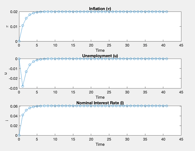
So, it’s been some days working on this but I don’t seem to get things right. I am completely new to Dynare. I am trying to solve a disinflation path numerically. I have tried to solve it as a stochastic simulation and now I am trying to do it as a foresight simulation. I have tried to set different initial values, tried to change the model… but still, my model seems off. I get initial inflation of zero that is stabilised then at 0.02. Unemployment starts at zero and then goes negative. I have also i starting at zero and stabilising itself at 0.06. I just think I might be telling the program the wrong initial values. Changing them (or even deleting u and i) doesn’t change anything. Any chance anyone know how to help?
Thanks in advance!
% 1. Declare the endogenous variables:
var pi u i;

% 2. Declare and set the parameters:
parameters beta pi_bar lambda xi kappa rho;

beta   = 0.96;
pi_bar = 0.02;
lambda = 0.75;
xi     = 0.2;             ´
kappa  = 10;
rho    = -log(beta);

% 3. Model Equations:
model;
    % (i) Phillips Curve:
    pi = lambda * pi(-1) + (1 - lambda)*pi_bar - xi * u;

    % (ii) Target Rule
    1 - exp(-u) = xi*kappa*(pi - pi_bar) + lambda*beta*(1 - exp(-u(+1)));

    % (iii) Euler Equation:
    i - u = rho + pi(+1) - u(+1);
end;

% 4. Initial values:
initval;
    % For a perfect foresight simulation these are our “guess” values for period 0.
    pi = 0.05;         % We set the time-0 value at the steady state (2%)
    u  = 0;
    i = rho + 0.05;
end;

% 5. Historical values:
histval;
    % Here, we force Dynare to “see” that prior to period 0, inflation was 5%.
    pi(-1) = 0.05;
end;

% 6. Steady State Calculations:
steady_state_model;
    u  = 0;
    pi = pi_bar;
    i  = rho + pi_bar;
end;

steady;
resid;

% 7. Perfect Foresight Simulation:
perfect_foresight_setup(periods = 40);
perfect_foresight_solver;

% 8. Plot the Simulation Results:
T = 0:(size(oo_.endo_simul,2)-1);

figure;
subplot(3,1,1);
plot(T, oo_.endo_simul(1,:)','-o');
title('Inflation (\pi)');
xlabel('Time');
ylabel('\pi');

subplot(3,1,2);
plot(T, oo_.endo_simul(2,:)','-o');
title('Unemployment (u)');
xlabel('Time');
ylabel('u');

subplot(3,1,3);
plot(T, oo_.endo_simul(3,:)','-o');
title('Nominal Interest Rate (i)');
xlabel('Time');
ylabel('i');

```