I recently went through the slides by Johannes Pfeifer on DSGE estimation (from the Kobe lectures).
I understand that basically the estimation proceeds in three steps:
Prior specification
Posterior maximization to find the mode
Posterior simulation via MCMC to get the entire distribution.
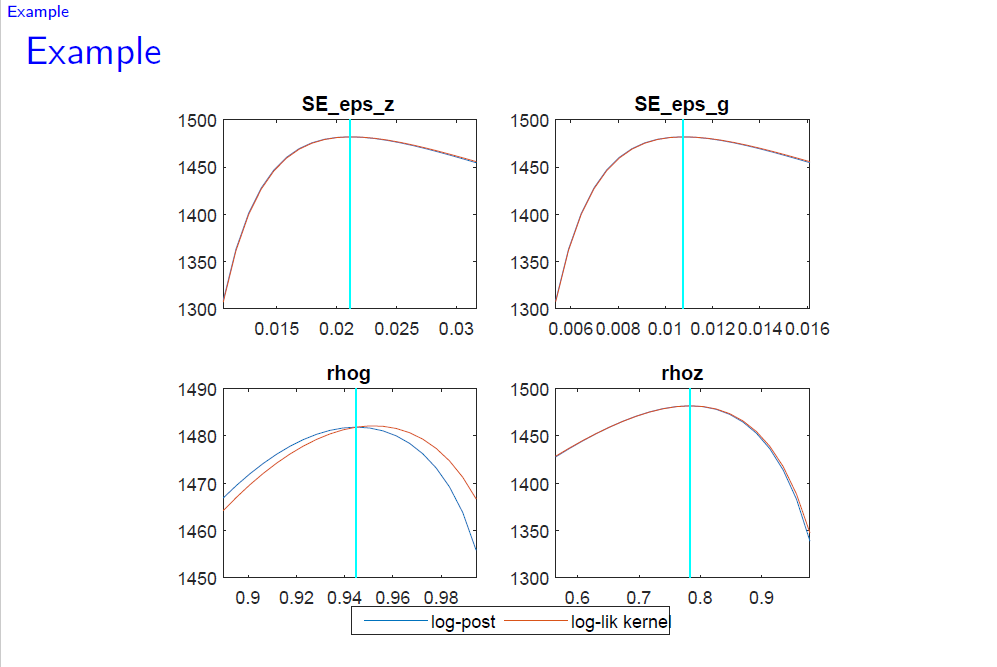
My question is: why do we need to simulate the posterior in step 3? From the mode_check plots, it seems as if we already have the posterior distribution?
In other words, what is the difference between the log-posterior stated in the mode_check plots and the posterior obtained via the MH algorithm. Why is the log-posterior not the one we are actually after?
After mode-finding, you have only one point of the posterior distribution: the mode. What you do not have is a full characterization of the posterior distribution. The mode_check-plots are only slices trough the posterior, i.e. a counterfactual of what would happen to the posterior density if you vary one parameter while keeping the others constant.
But you are interested in the density of the parameters in the posterior when they vary jointly. That is why you use the MCMC to trace out the full distribution.
Thank you for the quick response! I understand the plots better now!
So you are saying that for the mode computation, say of rhog, we vary the space of the parameter rhog from around 0.9 to 1, while keeping the other parameters fixed. So each parameter is fixed at their mode then?
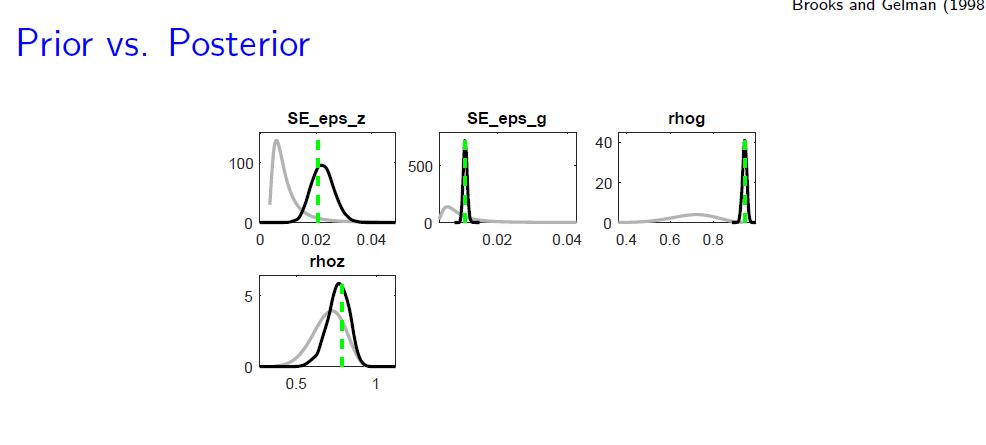
Moreover, when plotting the actual posterior distribution for rhog (obtained via the MH algorithm), what is the assumption on the other parameters? Are they kept fixed at their mode in this plot, while varying rhog?
I guess what i’m saying is: in both plots we only vary the space for one parameter and keep the others fixed somewhere, right? (I recognize that for the computation of the actual posterior, you allow for joint variation of the parameters in the MH algorithm.)
For the plots, we only have slices through highly dimensional objects. So everything else is kept fixed for the plots.
The main difference is what you show on the y-axis (the joint posterior in case of the mode_check-plots, the posterior density of the individual parameters for the prior-posterior plots)
Hi, I am not sure I understand correctly the last response by @jpfeifer. So I take the liberty of completing the answer. For the prior/posterior plots all the other parameters are varying. In these plots we compare marginal densities (prior density versus estimated posterior density). And, as you probably know, to obtain the marginal density out of a joint density we have to integrate w.r.t. the other parameters, which as a consequence cannot be held constant. In practice, to plot the estimated posterior density of, say rhog, we use all the draws for rhog in the metropolis simulation, without controlling the values of the other parameters (which take values as provided by the MCMC algorithm). If we were able to keep constant the other parameters (at the posterior mode for instance) we would estimate a conditional density.