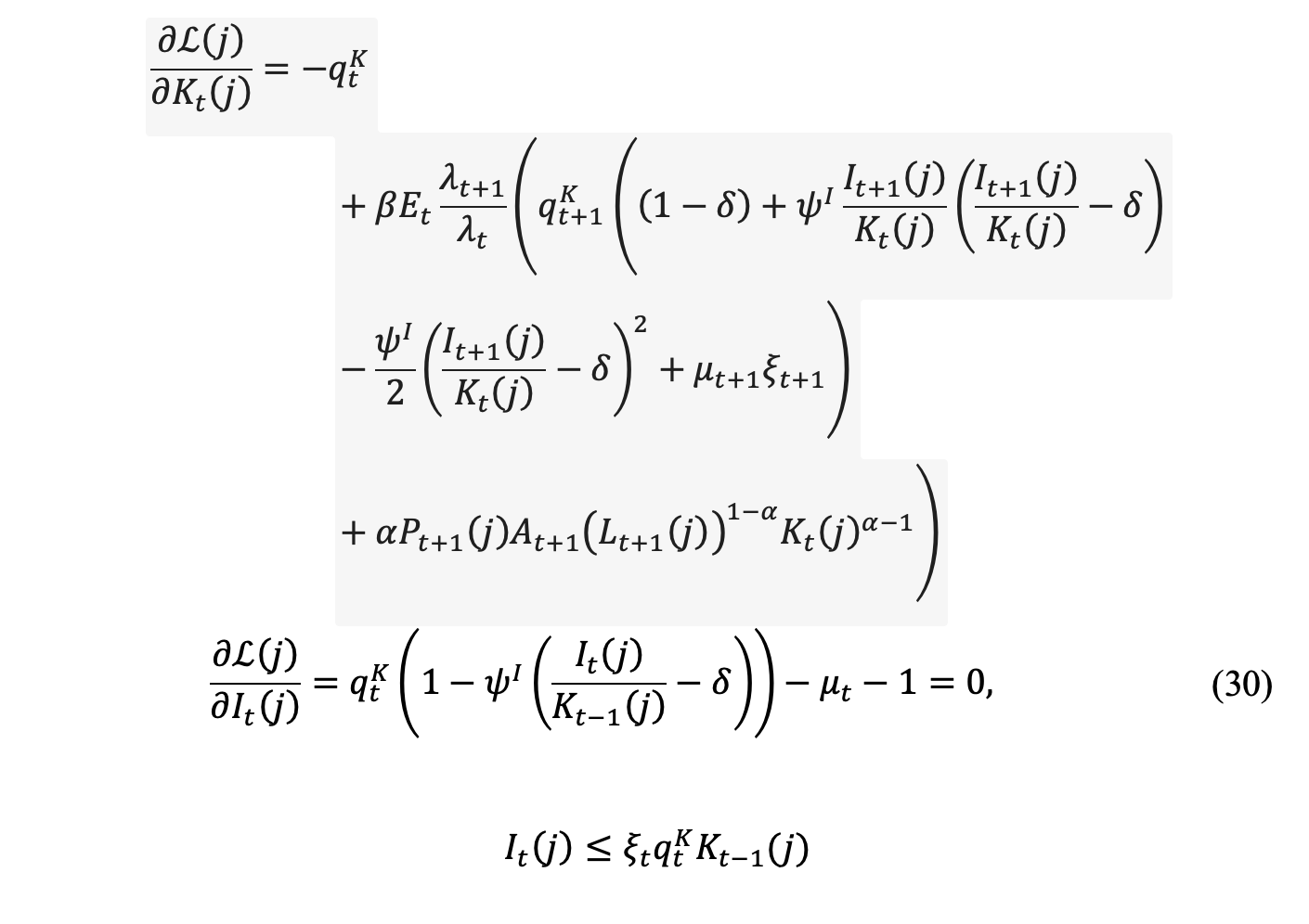
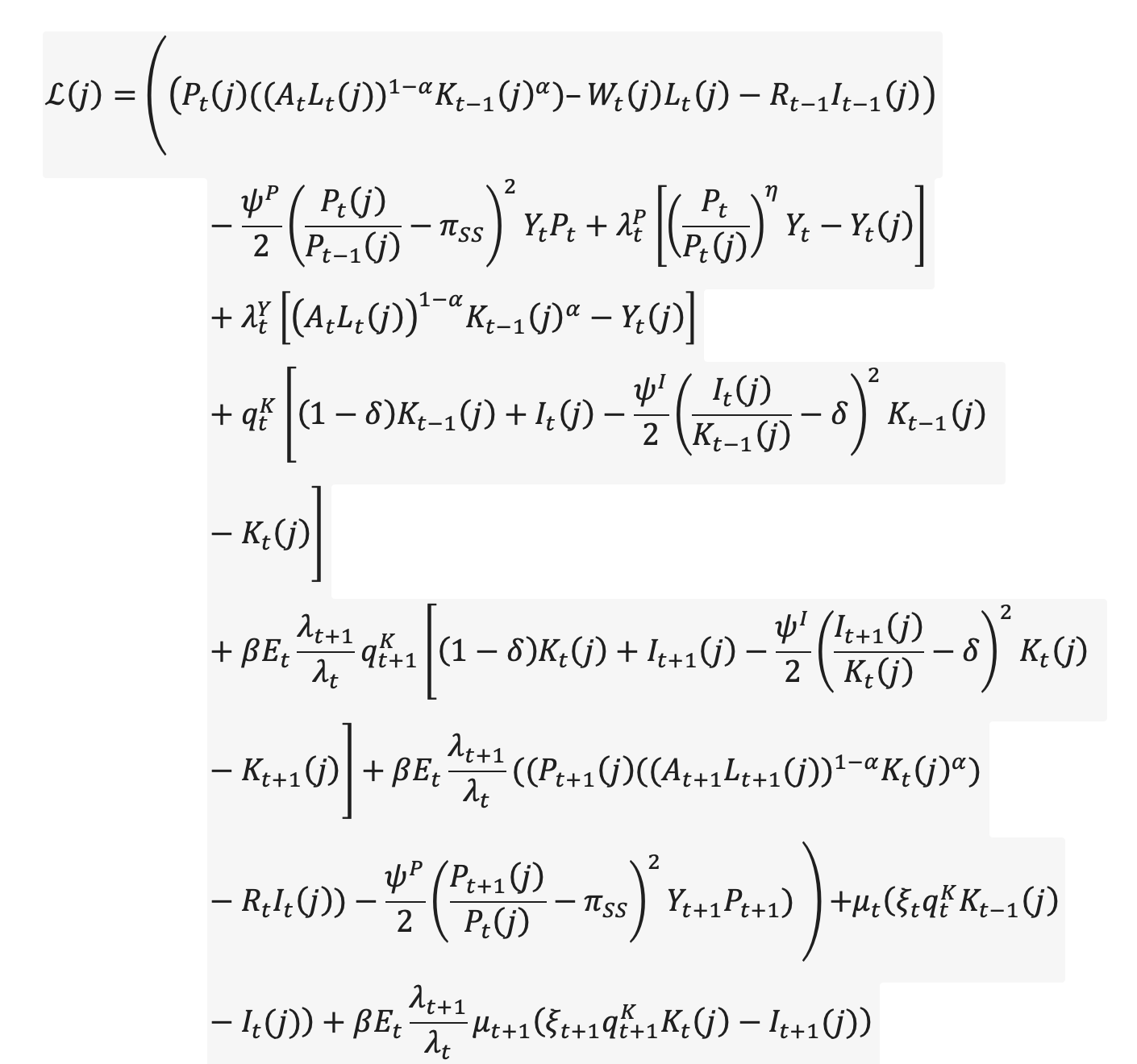
Thank you very much for your help! I have a question regarding detrending in DSGE models. I have the following Lagrangian, which is shown in the photo below. I don’t understand how to decompose (q^k_t) and (\mu_t) into trend and cycle components in order to perform the detrending process, and also (\xi_t) (which, in my opinion, should not have a trend).
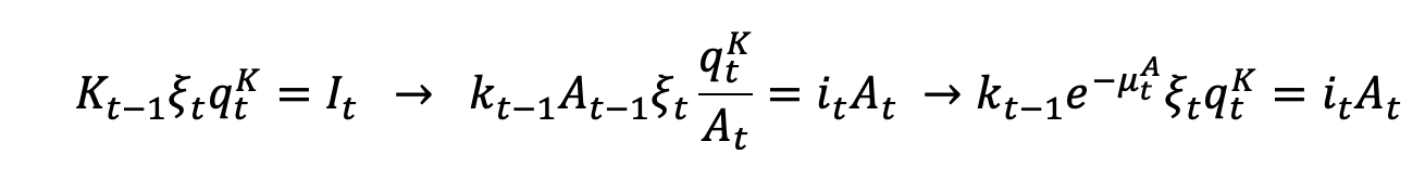
I also don’t know how to detrend these three FOCs for capital, investment, and the credit constraint (photo 2). Suppose that for investment, the decomposition into trend and cycle looks like (I_t = A_t \cdot i_t), and for capital (K_t = A_t \cdot k_t). But for these three variables, I don’t understand how to decompose them: (q^k_t) – the price of capital, (\mu_t) – the Lagrange multiplier for the credit constraint, and (\xi_t) – the borrowing limit. I model (A_t) as a non-stationary process.
The answer very much depends on the particular setup. See e.g. Tobin's Q - Capital Accumulation Constraint - #3 by diserable.
The price of capital is stationary if you define the multiplierr as q_t\times\lambda_t. Otherwise, It should have the same trend as \lambda_t. The borrowing limit should be stationary as it is defined as a fraction of capital.
Professor Pfeifer – initially, I treat (q_t^{K}) as the shadow price itself; I do not define it via multiplication with (\lambda_t). In the trend–cycle decomposition I use
\lambda_t^{\text{stat}} = \frac{\lambda_t}{A_t P_t},
and therefore
(q_t^{K})^{\text{stat}} = \frac{q_t^{K}}{A_t P_t}.
(I_t = A_t,i_t,; K_{t-1} = A_{t-1},k_{t-1},; P_t = P_t,p_t,; L_t = l_t). Substituting into the borrowing constraint yields
A_{t-1}k_{t-1},\xi_t,\frac{q_t^{K}}{A_t P_t} = A_t,i_t,
and multiplying through by (1/A_t) does not lead to a stationary representation.
To address this, I can redefine (Q_t = q_t^{K},\lambda_t). Then the borrowing constraint becomes
A_{t-1}k_{t-1},\xi_t,Q_t = A_t,i_t,
which, after multiplying by (1/A_t), yields a stationary form:
e^{-\mu^A_t},k_{t-1},\xi_t,Q_t = i_t.
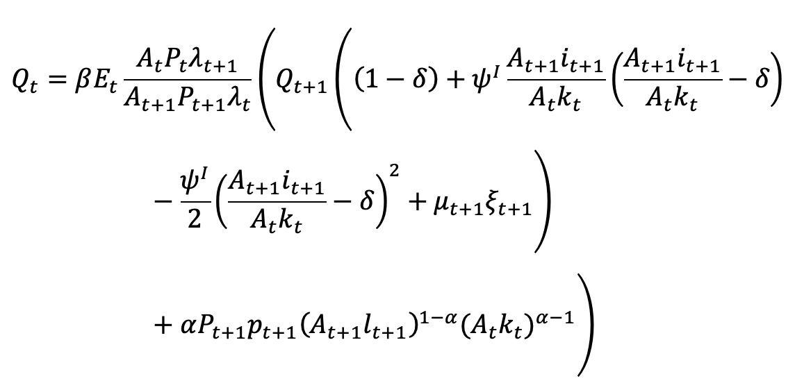
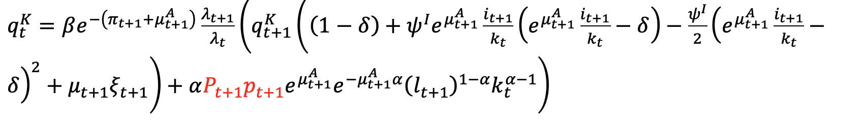
However, the situation changes when I consider the first-order condition with respect to capital. If I again assume (Q_t = q_t^{K},\lambda_t), I obtain
I conclude that (q^K_t) should not contain a trend; otherwise, stationarity cannot be achieved because the term (A_t) remains and cannot be canceled out.
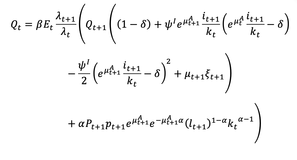
Assuming that ( q^K_t ) indeed has no trend, I obtain
In this equation, however, a trend remains in the term ( P_{t+1} p_{t+1} ).
Is my reasoning correct? And if so, what should I do about the remaining ( P_{t+1} p_{t+1} ) term – does it actually contain a trend, or are the prices themselves trendless?
It very much looks like you once applied the real stochastic discount factor to real variables and once to nominal ones. That causes such an inconsistency. The prices should drop out.
When solving the model, I did not apply detrending, and I am unsure whether this is an appropriate approach. For instance, Pt represents the price level, and with positive inflation (in my case, a target of 4% per year), it follows a unit root process. Could this choice significantly affect the results?
Additionally, I have a question regarding the collateral constraint: is it valid to include a constraint derived from a model without a trend into a model that does incorporate a trend?
The document you link considers a real model and therefore has a real stochastic discount factor. You instead have nominal and real constraints. That requires different discount factors depending on the type of constraint you are discounting.
Trend inflation is typically not a problem if you have complete indexing. If not, the model properties change. See e.g. Ascari/Sbordone (2014)'s JEL article.
Porting a constraint from a non trending model is fine as long as you know which variables inherit trends and that it still allows for stationarity after detrending.