Hello!
I am trying to estimate a fairly standard NK model with Calvo pricing, habit formation in consumption and flexible wages. The model derivation closely follows Ascari & Sbordone (2014), with the only major difference being that the Calvo parameter is endogenized as a function of current inflation. The model also includes government spending: my goal is to estimate the fiscal multiplier and see its interplay with endogenous price stickiness.
My prior setup is based on Smets & Wouters (2007). The problem is that none of the mode finders (except for mode_compute=6) seem to find the mode. All the other ones report a non-positive definite Hessian matrix. My questions are the following:
- Am I handling the data correctly? For all the variables in the dataset (see prepare_data) I take logs and multiply by 100. Then for trending variables (Y, C, G and N) I use the one-sided HP filter, while for inflation and interest rate I just use 100*log. In specifying the observation equations I was trying to follow the excellent guide on the topic.
- Am I handling parameter dependence correctly? I want to estimate steady-state interest rate and inflation rate. Together they determine the discount factor, which I specify in the steady_state_model block. This part is updated during estimation, isn’t it?
- Based on the identification command, I find that the weakest identification occurs for the parameters of the Taylor rule. Is this expected, given that the interest rate and the other two components of the Taylor rule are specified as observables, or am I missing something?
- I understand the restriction between the number of observed variables and shocks in the model. First, I started my estimation just based on Y_obs, R_obs, Pi_obs and G_obs. However, when I add other series (such as labour hours, for example), identification seems to improve. Is this a valid strategy of determining which data series to include into estimation?
- Could you please provide any advice on dealing with the non positive definite Hessian in my case? I don’t see any obvious mistakes with the model.
I enclose the zip file with code & data.
mod.zip (315.1 KB)
Any help/advice would be greatly appreciated!
I have slightly respecified the model (changed the preference specification to Jaimovich and Rebelo (2008)) and was still trying to debug the mode-finding process. So far I have:
- Made an exact replication of the Smets & Wouters data construction. I switched away from HP-filtered versions of variables to their demeaned growth rates. So my data is
100*log(R), 100*log(Pi) for stationary variables and 100*dlog(X) for Y, C and G. After computing the log differences I subtract the mean. Given that the correlations with SW’s original data is 0.99 for all the series (except for wages, probably due to later data revisions), I don’t think there are any problems on the data side. However, I would be glad for a confirmation.
- Rewritten the non-linear model without
exp()'ing all the variables. I have also redefined the observation equations and got rid of the erroneous multiplication by 100, which, as I realise, had been already dealt with by appropriate scaling of the shock standard errors. The observations equations now are:
    R_obs = log(R);
    Pi_obs = log(pai);
    Y_obs = log(Y/Y(-1)) + e_meY;
    C_obs = log(C/C(-1));
    G_obs = log(G/G(-1));
Is this specification correct, given my data and the rest of the model?
What puzzles me still is that during mode computation two of the persistence parameters seem to reach their upper bound of 0.99. I have seen posts on this forum suggesting that this is the model’s way of hinting about unit root behaviour. However, given that the data is in first differences, I don’t think this is the case. What could be the possible reason for this? Am I missing something?
mod.zip (407.0 KB)
I would be extremely grateful for any guidance!
The problem are
[quote=“Gulenkov, post:2, topic:27686”]
R_obs = log(R);
Pi_obs = log(pai);
In your Excel file, both variables still have a multiplication by 100. Their mean is about 1 in the data, but about 0 in the model.
1 Like
Yep, thanks a lot, that’s a silly mistake. So I removed the *100 multiplication from the excel file and started the mode computation again.
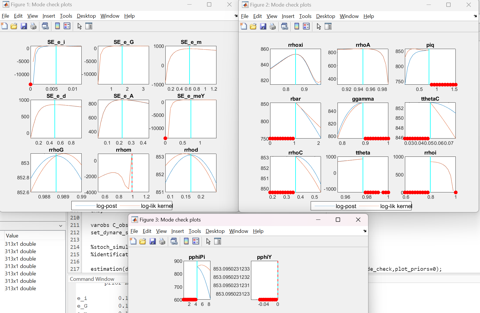
However, now even more parameters are at bounds, including Taylor rule coefficients, some persistence parameters and the Calvo share (approaching 1):
A first step is investigating what the red dots are.