i am novice.i need help from the seniors to run this mod.
welfare.xlsx (12.8 KB)
welfare2018.mod (11.0 KB)
i am novice.i need help from the seniors to run this mod.
welfare.xlsx (12.8 KB)
welfare2018.mod (11.0 KB)
What is the problem exactly when you run this model ?
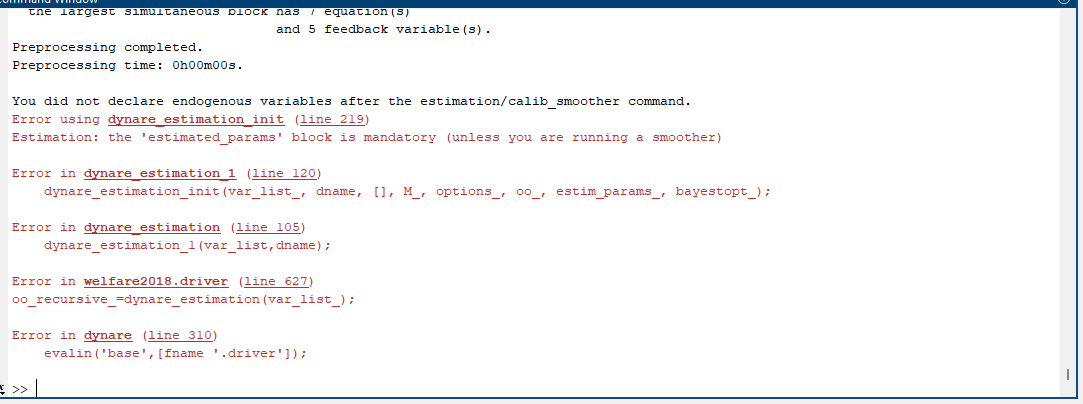
You did not declare estimated_params block in your mod file.
This block is mandatory when you estimate a DSGE model in dynare.
/*
/*
@#ifndef fixed_WPC_slope
@#define fixed_WPC_slope=0
@#endif
@#ifndef SGU_framework
@#define SGU_framework=0
@#endif
@#ifndef Calvo
@#define Calvo=1
@#endif
@#ifndef taxes
@#define taxes=0
@#endif
var pi_p {\pi^p} (long_name=‘price inflation’)
y_gap {\tilde y} (long_name=‘output gap’)
y_nat {y^{nat}} (long_name=‘natural output’) //(in contrast to the textbook defined in deviation from steady state)
y {y} (long_name=‘output’)
yhat {\hat y} (long_name=‘output deviation from steady state’)
r_nat {r^{nat}} (long_name=‘natural interest rate’)
r_real {r^r} (long_name=‘real interest rate’)
i {i} (long_name=‘nominal interrst rate’)
n {n} (long_name=‘hours worked’)
m_real {(m-p)} (long_name=‘real money stock’)
m_growth_ann {\Delta m} (long_name=‘money growth annualized’)
m_nominal {m} (long_name=‘nominal money stock’)
nu {\nu} (long_name=‘AR(1) monetary policy shock process’)
a {a} (long_name=‘AR(1) technology shock process’)
r_real_ann {r^{r,ann}} (long_name=‘annualized real interest rate’)
i_ann {i^{ann}} (long_name=‘annualized nominal interest rate’)
r_nat_ann {r^{nat,ann}} (long_name=‘annualized natural interest rate’)
pi_p_ann {\pi^{p,ann}} (long_name=‘annualized inflation rate’)
z {z} (long_name=‘AR(1) preference shock process’)
p {p} (long_name=‘price level’)
w {w} (long_name=‘nominal wage’)
c {c} (long_name=‘consumption’)
w_real \omega (long_name=‘real wage’)
w_gap {\tilde \omega} (long_name=‘real wage gap’)
pi_w {\pi^w} (long_name=‘wage inflation’)
w_nat {w^{nat}} (long_name=‘natural real wage’)
mu_p {\mu^p} (long_name=‘markup’)
pi_w_ann {\pi^{w,ann}} (long_name=‘annualized wage inflation rate’)
;
varexo eps_a {\varepsilon_a} (long_name=‘technology shock’)
eps_nu {\varepsilon_\nu} (long_name=‘monetary policy shock’)
eps_z {\varepsilon_z} (long_name=‘preference shock innovation’)
;
parameters alppha {\alpha} (long_name=‘capital share’)
betta {\beta} (long_name=‘discount factor’)
rho_a {\rho_a} (long_name=‘autocorrelation technology shock’)
rho_nu {\rho_{\nu}} (long_name=‘autocorrelation monetary policy shock’)
rho_z {\rho_{z}} (long_name=‘autocorrelation demand shock’)
siggma {\sigma} (long_name=‘inverse EIS’)
varphi {\varphi} (long_name=‘inverse Frisch elasticity’)
phi_pi {\phi_{\pi}} (long_name=‘inflation feedback Taylor Rule’)
phi_y {\phi_{y}} (long_name=‘output feedback Taylor Rule’)
eta {\eta} (long_name=‘semi-elasticity of money demand’)
epsilon_p {\epsilon_p} (long_name=‘demand elasticity goods’)
theta_p {\theta_p} (long_name=‘Calvo parameter prices’)
epsilon_w {\epsilon_w} (long_name=‘demand elasticity labor services’)
@#if Calvo
theta_w {\theta_w} (long_name=‘Calvo parameter wages’)
@#else
phi_w {\phi_w} (long_name=‘Rotemberg parameter wages’)
@#endif
tau {\tau} (long_name=‘labor subsidy’)
lambda_w {\lambda_w} (long_name=‘Slope of the wage PC’)
tau_n_SS {bar {\tau^n}} (long_name=‘Steady state labor tax’)
;
%----------------------------------------------------------------
% Parametrization, p. 67 and p. 113-115
%----------------------------------------------------------------
siggma = 1;
varphi=5;
phi_pi = 1.5;
phi_y = 0.125;
theta_p=3/4;
rho_nu =0.5;
rho_z = 0.5;
rho_a = 0.9;
betta = 0.99;
eta =3.77; %footnote 11, p. 115
alppha=1/4;
epsilon_p=9;
tau=0; //1/epsilon_p;
epsilon_w=4.5;
@#if fixed_WPC_slope
lambda_w=0.03;
@#else
theta_w=3/4;
@#endif
@#if taxes
tau_n_SS=0.99;
@#else
tau_n_SS=0;
@#endif
%----------------------------------------------------------------
% First Order Conditions
%----------------------------------------------------------------
model(linear);
//Composite parameters
#Omega=(1-alppha)/(1-alppha+alpphaepsilon_p); %defined on page 166
#psi_n_ya=(1+varphi)/(siggma(1-alppha)+varphi+alppha); %defined on page 171
#psi_n_wa=(1-alpphapsi_n_ya)/(1-alppha); %defined on page 171
#lambda_p=(1-theta_p)(1-bettatheta_p)/theta_pOmega; %defined on page 166
#aleph_p=alpphalambda_p/(1-alppha); %defined on page 172
#aleph_w=lambda_w(siggma+varphi/(1-alppha)); %defined on page 172
[name=‘New Keynesian Phillips Curve eq. (18)’]
pi_p=bettapi_p(+1)+aleph_py_gap+lambda_pw_gap;
[name=‘New Keynesian Wage Phillips Curve eq. (22)’]
pi_w=bettapi_w(+1)+aleph_wy_gap-lambda_ww_gap;
[name=‘Dynamic IS Curve eq. (22)’]
y_gap=-1/siggma*(i-pi_p(+1)-r_nat)+y_gap(+1);
[name=‘Interest Rate Rule eq. (26)’]
i=phi_pipi_p+phi_yyhat+nu;
[name=‘Definition natural rate of interest eq. (24)’]
r_nat=-siggmapsi_n_ya(1-rho_a)a+(1-rho_z)z;
[name=‘Definition wage gap, eq (21)’]
w_gap=w_gap(-1)+pi_w-pi_p-(w_nat-w_nat(-1));
[name=‘Definition natural wage, eq (16)’]
w_nat=psi_n_waa;
[name=‘Definition markup’]
mu_p=-alppha/(1-alppha)y_gap-w_gap;
[name=‘Definition real wage gap, p. 171’]
w_gap=w_real-w_nat;
[name=‘Definition real interest rate’]
r_real=i-pi_p(+1);
[name=‘Definition natural output, eq. (20)’]
y_nat=psi_n_yaa;
[name=‘Definition output gap’]
y_gap=y-y_nat;
[name=‘Monetary policy shock’]
nu=rho_nunu(-1)+eps_nu;
[name=‘TFP shock’]
a=rho_aa(-1)+eps_a;
[name=‘Production function, p. 171’]
y=a+(1-alppha)n;
[name=‘Preference shock, p. 54’]
z = rho_zz(-1) - eps_z;
[name=‘Money growth (derived from eq. (4))’]
m_growth_ann=4(y-y(-1)-eta*(i-i(-1))+pi_p);
[name=‘Real money demand (eq. 4)’]
m_real=y-etai;
[name=‘Annualized nominal interest rate’]
i_ann=4i;
[name=‘Annualized real interest rate’]
r_real_ann=4r_real;
[name=‘Annualized natural interest rate’]
r_nat_ann=4r_nat;
[name=‘Annualized inflation’]
pi_p_ann=4pi_p;
[name=‘Annualized wage inflation’]
pi_w_ann=4pi_w;
[name=‘Output deviation from steady state’]
yhat=y-steady_state(y);
[name=‘Definition price level’]
pi_p=p-p(-1);
[name=‘resource constraint, eq. (12)’]
y=c;
[name=‘definition real wage’]
w_real=w-p;
[name=‘definition real wage’]
m_nominal=m_real+p;
end;
%----------------------------------------------------------------
% define shock variances
%---------------------------------------------------------------
shocks;
var eps_nu = 0.25^2; //1 standard deviation shock of 25 basis points, i.e. 1 percentage point annualized
var eps_a = 1^2; //unit shock to technology
var eps_z = 1^2; //unit shock to technology
end;
%----------------------------------------------------------------
% steady states: all 0 due to linear model
%---------------------------------------------------------------
steady_state_model;
@#if fixed_WPC_slope
%keep fixed slope of WPC and compute parameters accordingly
@#if SGU_framework
@#if Calvo
theta_w=get_Calvo_theta(lambda_w,epsilon_w,betta,varphi,1);
@#else
phi_w=(epsilon_w-1)(1-tau_n_SS)/lambda_w(1-alppha)(epsilon_p-1)/epsilon_p/tau_s_ptau_s_w;
@#endif
@#else
@#if Calvo
theta_w=get_Calvo_theta(lambda_w,epsilon_w,betta,varphi,0);
@#else
phi_w=(epsilon_w-1)(1-tau_n_SS)/lambda_w(1-alppha)(epsilon_p-1)/epsilon_p/tau_s_ptau_s_w;
@#endif
@#endif
@#else
@#if SGU_framework
%compute slope (and ) based on Calvo parameter
@#if Calvo
lambda_w=(1-theta_w)(1-bettatheta_w)/theta_w;
@#else
phi_w=(epsilon_w-1)/((1-theta_w)(1-bettatheta_w))(1-tau_n)theta_w(1-alppha)(epsilon_p-1)/epsilon_p/tau_s_ptau_s_w;
lambda_w=(epsilon_w-1)/phi_w(1-tau_n)(1-alppha)(epsilon_p-1)/epsilon_p/tau_s_ptau_s_w;
@#endif
@#else
@#if Calvo
lambda_w=(1-theta_w)(1-bettatheta_w)/(theta_w(1+epsilon_wvarphi));
@#else
phi_w=(epsilon_w-1)/((1-theta_w)(1-bettatheta_w))(1-tau_n)theta_w(1-alppha)(epsilon_p-1)/epsilon_p/tau_s_ptau_s_w*(1+epsilon_wvarphi);
lambda_w=(epsilon_w-1)(1-tau_n)/phi_w*(1-alppha)(epsilon_p-1)/epsilon_p/tau_s_ptau_s_w;
@#endif
@#endif
@#endif
end;
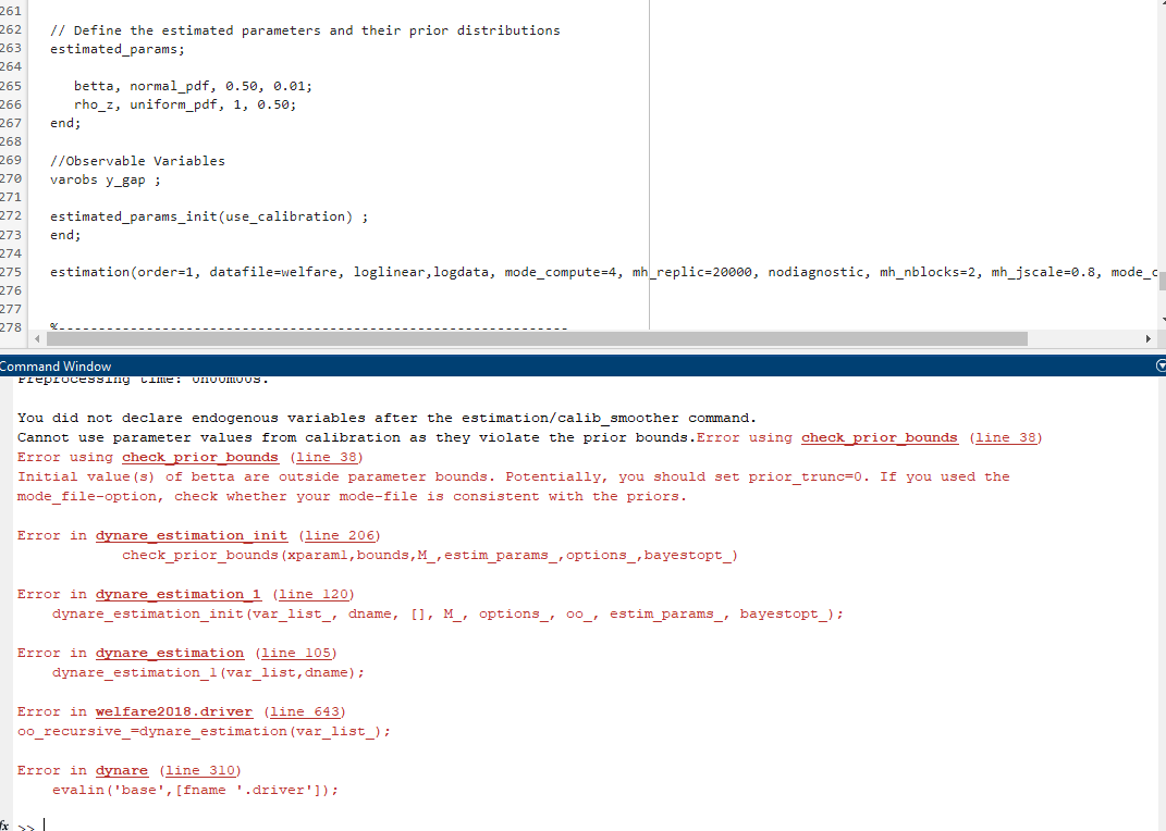
// Define the estimated parameters and their prior distributions
estimated_params;
betta, normal_pdf, 0.50, 0.01;
rho_z, uniform_pdf, 1, 0.50;
% Define other parameters to estimate…
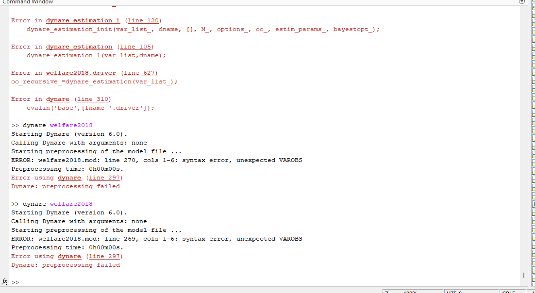
//Observable Variables
varobs y_gap ;
estimation(order=1, datafile=welfare, loglinear,logdata, mode_compute=4, mh_replic=20000, nodiagnostic, mh_nblocks=2, mh_jscale=0.8, mode_check);
%----------------------------------------------------------------
% generate IRFs for monetary policy shock
%----------------------------------------------------------------
stoch_simul(order = 1,irf=15) y_gap pi_p_ann pi_w_ann w_real y n;
still doesnt work
When you use estimated_params block at the end of this block you should use end;
estimated_params;
betta, normal_pdf, 0.50, 0.01;
rho_z, uniform_pdf, 1, 0.50;
end;
Use this block in your model before the estimation command.
estimated_params_init(use_calibration) ;
end;
And then run the model again.
After the estimation command write endogenous variables names. For example y i c n after the estimation command.
In DSGE models do not use i for investment and use I or Inv or inv .
Do not use MATLAB built-in functions names or similar MATLAB command names because MATLAB may cause problem when you solve the model.
i do not get you.could you please check my mod.i am sharing here again.
welfare2018.mod (11.2 KB)
welfare.xlsx (12.8 KB)
After the estimation command write endogenous variables names for example:
estimation( …) y i c n ;
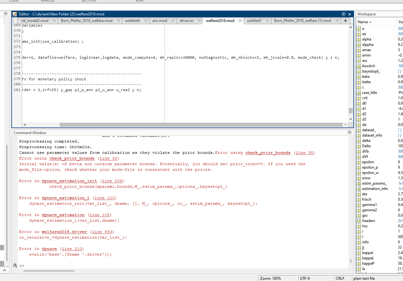
As the message states, you use
estimated_params_init(use_calibration) ;
end;
to start at beta=0.99. But you set
estimated_params;
   betta, normal_pdf, 0.50, 0.01;
With a having a 49 standard deviation difference to the mean of the specified distribution is virtually impossible.
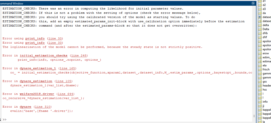
I still don’t know what you are trying to do. But you cannot use the loglinear option in your model due to negative/zero steady states.
Alright Professor.