Hello everyone, Please help me out with the following.
In NK models, the (FOCs) equations for factors demand by the individual (monopolistically competitive) intermediate firms INCLUDE marginal cost. We basically have something like this:
1.Y = Y(K, L, KG) : Production function
2. K = a.MC.(Y/R) : Dde for K
3. L = (1-a).MC.(Y/W) : Dde for L
These three equations fixe K, L and MC (Y comes from the Demand side).
Now, we could derive the MC equation but it would be REDUNDANT unless we replace one of the three original equations with it.
However, Dynare doesn’t work with the above theoretical system (no matter what variation of it)!
Instead, (as can be seen from the code in the following thread Theoretical Moments: NaN - #3 by kofiemma), Celso in his book used the following (weird) modification to get the code to work:
1.Y = Y(K, L, KG) : Production function
2. K = a.(Y/R) : Dde for K
3. L = (1-a).(Y/W) : Dde for L
4. MC = MC(R, W) : Derived MC equation
He removed MC from factor demand equations and added the MC equation to the system.
This works (I safely remove 1 other equation from the whole model) but it looks like the setting for Perfectly Competitive firms and more importantly CANNOT be derived from the program of the NK intermediate firm (I’ve tried a lot!).
What should I do? What is wrong with Dynare and the first system? Is it safe to use to second system ?
I am not sure I get the point. What do you mean with redundant? We have
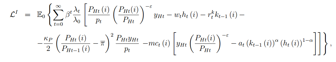
\mathcal{L} = {Y_t} - {w_t}{N_t} - {R_t}{K_t} - m{c_t}\left( {{Y_t} - {A_t}K_t^\alpha L_t^{1 - \alpha }} \right) \\
\frac{{\partial \mathcal{L}}}{{\partial {Y_t}}} = 1 - m{c_t} = 0 \Rightarrow m{c_t} = 1
So marginal cost in the RBC model is equal to 1.
Thank you for your answer.
I understand real mc in RBC should be 1. But the above is about an NK model with price setting intermediate firms and a Taylor rule, so I am working with a Nominal MC here and real mc is kinda irrelevant. Is the nominal MC equation not redundant in the case described above?
I loglinearized the model and the first system above finally worked really well. Maybe it is because the raw model is highly nonlinear that Dynare is having trouble with it.
Anyways, I am happy I made it through the complexity of this model. I will be uploading my code here when I finalise it
I don’t think it is because of the log linearisation. When you log linearised a model by hand or enter the nonlinear version in dynare, you get the same dynamics. So maybe you should look again at your model…
So the model includes monopolistically competitive intermediate firms and Calvo pricing.
Thus the aggregate demand comes from the resource constraint and is a function of aggregate price. The final firm’s problem generates the individual demands for intermediate goods (Y above) which is a function of individual prices charges by the respective firms.
The intermediate firms above then take individual demands as given and and choose prices (in a second step following the above) considering the probability of not updating their prices in the future.
So Yi=Yi(Pi) and Pi is determined later.
I hope it makes sense like this
Very good observation. The Nonlinear model has finally worked.
I was confused by how the wholesale firm’s program is presented by some papers.
It usually is in two steps: First cost minimisation to determine factor demands (and marginal cost) and Second profit maximisation to determine optimal price.
But I set the whole Calvo problem as a single dynamic maximisation one and systematically obtained a general set of FOCs determining optimal price, L multiplier (nominal MC) and factor demands.
So the redundancy problem went away.
Yes the second setup is similar to the above.
It’s just like I pointed out in my first post. After taking the derivatives and writing out the FOCs I still worked out the total cost function and then the nominal marginal cost (as a function of nominal W and R) which I added to the initial FOCs system. I then twisted the whole code to get it to work (it looked weird but as I said, I was a little confused by the two steps problem).
And btw, I still need to approximate the optimal price equation (which includes an infinite sum of future nominal marginal costs) for dynare to find the Nonlinear steady state (used in the DSGE literature). If i just keep it like it is and write it as recursive in the numerator and denominator then the Nonlinear steady state can’t be computed by dynare even if the sum of residual is around 0.02. So I guess loglinearizing was particularly necessary in this case to avoid having to approximate the said equation
I also don’t see the point. How is providing a steady state for the non-linear version different than having the same steady state to approximate around?
Oh I should’ve said ‘‘Simplify’’ instead. The opt. price was something like Infinite_Sum(P.Y.MC)/Infinite_Sum(P.Y) and I had to simplify it as Infinite_Sum(MC) for dynare to somehow compute the Nonlinear steady state.
Of course I manually calculated the steady state of the model and used it as initial guess but dynare still couldn’t find the steady state of the Nonlinear model from those values (unless if I make the above simplification).
Btw I don’t have a Phillips curve equation but I used the two separate equations for optimal price (as a function of MC) and general price level (as a function of its lag and optimal price).