Combining IRFs derived under different parameter values on a single plot

Julie · February 16, 2023, 12:02pm

Hi Professor,

I am wondering

is there any quicker way to combine IRFs derived under different sets of parameter values on a single plot? I experimented a bit myself using the “set_param_value” function, starting from the SWUS dynare file, but it didn’t seem to work. I know I can manually save IRFs derived under one set of parameters as mat files, and then combine them, but I am wondering if I can achieve this in one go?

please find attached my model file “test.mod”, where I have added “set_param_value” on lines 46-47, and also lines 277-287 within the plotting block. Could you help me with this?

when plotting IRFs with Matlab derived by Dynare, is it possible to write loops like for i=1:10, plot (:,1)… so that I don’t need to repeat those code for each variable as I am currently doing?
In other words, I want to know if it’s possible to optimize lines 272-779?

Thanks for your help in advance!
test.mod (18.2 KB)

jpfeifer · February 16, 2023, 4:01pm

The essential logic is:

set_param_value('calfa',0.1);
set_param_value('cbeta',0.5);
stoch_simul(noprint,nofunctions,nograph,nomoments,nocorr,irf=50,irf_shocks=(ea eb eg eqs em epinf ew))r inve pk kp pinf w c y lab rk;
IRFs1=oo_.irfs;

set_param_value('calfa',0.3);
set_param_value('cbeta',1.2);
stoch_simul(noprint,nofunctions,nograph,nomoments,nocorr,irf=50,irf_shocks=(ea eb eg eqs em epinf ew))r inve pk kp pinf w c y lab rk;
IRFs2=oo_.irfs;


figure('Name','shock1_eat')

var_names={'r','inve'}
var_titles={'Interest rate','Investment'}

for var_iter=1:length(var_names)
    subplot(3,5,var_iter)
    plot([1:options_.irf],IRFs1.([var_names{var_iter} '_ea']),'b-','LineWidth',1.5)
    hold on
    plot([1:options_.irf],IRFs2.([var_names{var_iter} '_ea']),'b-','LineWidth',1.5)
    ylabel('productivity shock')
    title(var_titles{var_iter})
    if var_iter==1
        legend('a=0.5,b=0.2','a=0.7,b=0.3');
    end
end

Julie · February 16, 2023, 5:19pm

Wonderful solution!!!

The reason you used “if var_iter==1” in the end was because you wanted to have one legend only on the first subplot, correct?

Julie · February 16, 2023, 6:49pm

Another question is that:
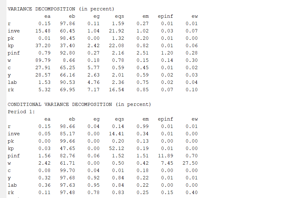
When I used command: stoch_simul(order=1,conditional_variance_decomposition=[1,4,8,16,40], periods=0, nograph,irf_shocks=(ea eb eg eqs em epinf ew))r inve pk kp pinf w c y lab rk;
to calculate variance decomposition, I obtained results for variance decomposition and conditional variance decomposition, and the results displayed in the results window are similar.

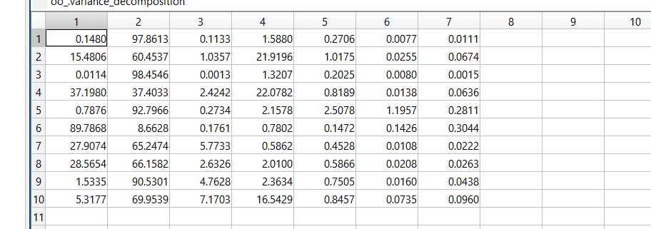
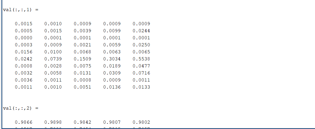
However, when I clicked on oo_variance_decompositon and oo_conditional_variance_decomposition, I found the matrix for variance decomposition looks exactly the same as it is in the results window,

while that for conditional variance looks very different …so what caused such inconsistency？ If I want to plot conditional variance decomposition using bar chart, where could I find the result as displayed in the result window?

jpfeifer · February 17, 2023, 4:00pm

Yes, that is because I only want the legend for the first variable.
Have a look at the manual. It documents the three dimensional array:

https://www.dynare.org/manual/the-model-file.html?highlight=oo_%20conditional_variance_decomposition#oo_.conditional_variance_decomposition

Julie · February 19, 2023, 1:34pm

MATLAB/Octave variable: oo_.conditional_variance_decomposition ¶

After a run of stoch_simul with the conditional_variance_decomposition option, contains a three-dimensional array with the result of the decomposition. The first dimension corresponds to the endogenous variables (in the order of declaration after the command or in M_.endo_names if not specified), the second dimension corresponds to the forecast horizons (as declared with the option), and the third dimension corresponds to the exogenous variables (in the order of declaration). In the presence of measurement error, the field will contain the variance contribution after measurement error has been taken out, i.e. the decomposition will be conducted of the actual as opposed to the measured variables.

Yes, I have found the explanation from the manual, but how am I supposed to create a stacked bar plot for say variance decomposition for 1-period horizon?

It’s not difficult to do so for variance decomposition (e.g. figure
ba=bar(oo_.variance_decomposition, ‘stacked’,‘FaceColor’,‘flat’), since the results are stored as a number of variables specified*number of shocks two-dimensional matrix. but I have no clue how to do that with the 3-dimensional matrix.

The second question is how to export the historical shock decomposition results into a excel file? after using the following command to conduct historical shock decomposition?

shock_groups(name=group1);

‘price mark up(epinf)’= epinf;
‘wage mark up (ew)’= ew;
‘productitivity’= ea;
‘government spending’= eg;
‘others’=em, eb, eqs;
end;

shock_decomposition (use_shock_groups=group1)y;

Many thanks!

jpfeifer · February 19, 2023, 10:31pm

You can take a horizon and then use squeeze in Matlab to eliminate the singular horizon dimension, i.e. get a two-dimensional matrix.
@rattoma is the one to ask.

Julie · February 20, 2023, 8:50pm

Hi Prof,

I have tried the squeeze function and obtained the desired results.
But I am now stuck with making values appear in the center of bars.


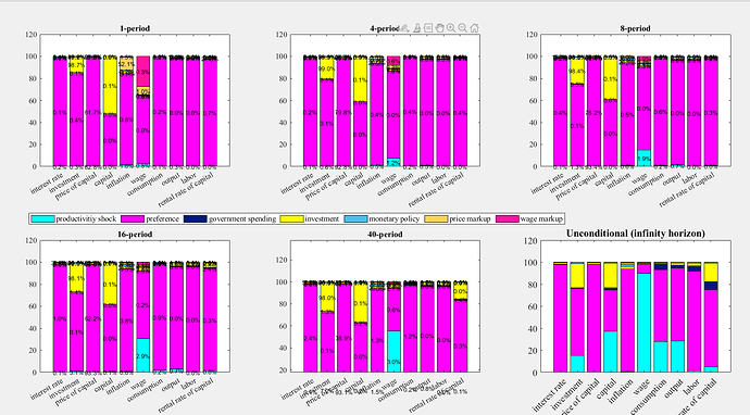
     figure('Name','Conditional and unconditional variance decomposition')
	 horizon_titles={'1-period','4-period','8-period','16-period','40-period'};
	  
	  
  for k=1:size(oo_.conditional_variance_decomposition,2)
	  subplot(2,3,k)
	  
      ba=bar(squeeze(oo_.conditional_variance_decomposition(:,k,:)*100),'stacked','FaceColor','flat');
      ba(:,1).CData=[0     1     1];
      ba(:,2).CData=[1     0     1];
      ba(:,3).CData=[0.0  0.1  0.5];
      ba(:,4).CData=[1     1      0];
      ba(:,5).CData=[0.3020    0.7451    0.9333];
      ba(:,6).CData=[0.9882    0.8314    0.3569];
      ba(:,7).CData=[1.0000    0.0745    0.6510];
	  
		 	
	//for g=1:7
	// ba(:,g).FaceAlpha = .6;      % adding opacity
	// end;

   
    vd_2d=squeeze(oo_.conditional_variance_decomposition(:,k,:))*100;

    if any(vd_2d>0.3) 
      xbarCnt = vertcat(ba.XEndPoints); 
      ybarTop = vertcat(ba.YEndPoints);
      ybarCnt = ybarTop - vd_2d/2;
      txt = compose('%.1f%%',vd_2d);
      th = text(xbarCnt(:), ybarCnt(:), txt(:),'HorizontalAlignment', 'center', ....
      'VerticalAlignment', 'middle', 'Color', 'k','FontSize', 8);
	  else;
    end

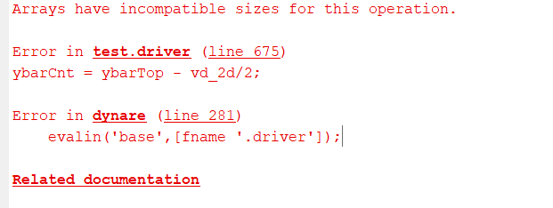
The code above returned a error message saying:

but it’s modified based on a solution to a very similar question:

And using:

x = 1:5; 
rng('default') % for reproducibility
y = rand(4,5) * 10;  
h =  bar(x, y,'stacked'); 
% Compute percentage
yp = y./sum(y) * 100; 
% Compute bar segment centers
xbarCnt = vertcat(h.XEndPoints); 
ybarTop = vertcat(h.YEndPoints);
ybarCnt = ybarTop - y/2; 
% Create text strings
txt = compose('%.1f%%',yp);
% Add text 
th = text(xbarCnt(:), ybarCnt(:), txt(:), ...
    'HorizontalAlignment', 'center', ....
    'VerticalAlignment', 'middle', ...
    'Color', 'w',....
    'FontSize', 8);

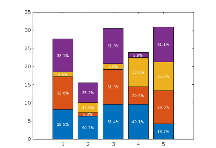
I can obtain:

PS: I also attempted to also add a threshold so it’s the number<a, it won’t appear inside the bar.
Please could you let me know how to fix this? ( how to correctly calculate the position for the texts here)

Best

jpfeifer · February 24, 2023, 3:06pm

This looks like more like Matlab support than Dynare support. This is unfortunately not my area of expertise. In any case, you did not provide a full code to replicate the issue.

Julie · February 25, 2023, 12:46pm

Hi Professor,

Thanks for your reply.
test1.mod (11.8 KB)
Here is the code file.

jpfeifer · February 27, 2023, 7:17pm

It seems there is a transpose missing. Try

      ybarCnt = ybarTop - vd_2d'/2;

Julie · February 28, 2023, 7:23am

The code works this time, but the result does not look right…I don’t think the numbers appear in the right place for the individual bar segments they correspond to.

jpfeifer · February 28, 2023, 10:32pm

Try with a consistent transpose:


figure('Name','Conditional and unconditional variance decomposition')
horizon_titles={'1-period','4-period','8-period','16-period','40-period'};


for k=1:size(oo_.conditional_variance_decomposition,2)
    subplot(2,3,k)

    ba=bar(squeeze(oo_.conditional_variance_decomposition(:,k,:)*100),'stacked','FaceColor','flat');
    ba(:,1).CData=[0     1     1];
    ba(:,2).CData=[1     0     1];
    ba(:,3).CData=[0.0  0.1  0.5];
    ba(:,4).CData=[1     1      0];
    ba(:,5).CData=[0.3020    0.7451    0.9333];
    ba(:,6).CData=[0.9882    0.8314    0.3569];
    ba(:,7).CData=[1.0000    0.0745    0.6510];

    vd_2d=squeeze(oo_.conditional_variance_decomposition(:,k,:))'*100;

    if any(vd_2d>0.3)
        xbarCnt = vertcat(ba.XEndPoints);
        ybarTop = vertcat(ba.YEndPoints);
        ybarCnt = ybarTop - vd_2d/2;
        txt = compose('%.1f%%',vd_2d);
        th = text(xbarCnt(:), ybarCnt(:), txt(:),'HorizontalAlignment', 'center', ....
            'VerticalAlignment', 'middle', 'Color', 'k','FontSize', 8);
    else;
    end


    xticklabels({'interest rate','investment','price of capital','capital','inflation','wage','consumption','output','labor','rental rate of capital'});
    ylim([0 120]);
    title(horizon_titles{k})
    set(gca,'FontSize',10, 'FontName','Times','FontWeight','normal');

    if k==1
        Lgnd=legend('productivitiy shock','preference','government spending','investment','monetary policy','price markup','wage markup');
        set(Lgnd, 'FontSize',10,'FontWeight','Normal','FontName','Times','Orientation','horizontal');
    end

end