Chari_et_al_2007.mod

Hi Prof. Pfeifer,

May I ask which utility function you used in your BCA replication of Chari et. al paper. From euler equation in the mod file,
(1+{{\tau_x}_{t}}) ({{c}_{t}})^{(-{{\sigma}})} (1-({{l}_{t}}))^{{{\psi}} (1-{{\sigma}})}={{\hat \beta}} ({{c}_{t+1}})^{(-{{\sigma}})} (1-({{l}_{t+1}}))^{{{\psi}} (1-{{\sigma}})} ((1-{{\delta}}) (1+{{\tau_x}_{t+1}})+(({{l}_{t+1}}) ({{z}_{t+1}}))^{1-{{\theta}}} {{\theta}} ({{k}_{t}})^{{{\theta}}-1})
it seems U = \frac{{{c}_{t}}^{(1-{{\sigma}})} }{1-{{\sigma}}} (1-({{l}_{t}}))^{{{\psi}}\, (1-{{\sigma}})}.

But that suggests the following intratemporal condition: \frac{{{\psi}}\, \left({{c}_{t}}\right)^{{{}}}}{1-\left({{l}_{t}}\right)}=\left(1-{{\tau_l}_{t}}\right)\, \left({{w}_{t}}\right) . And not \frac{{{\psi}}\, \left({{c}_{t}}\right)^{{{\sigma}}}}{1-\left({{l}_{t}}\right)}=\left(1-{{\tau_l}_{t}}\right)\, \left({{w}_{t}}\right) used in the mod file. It does not affect the results though. But is this the utility function you used for the replication?

Also, you use the following law of motion for capital;
\left(1+\gamma_{z}\right)\left(1+\gamma_{n}\right)\left(k_{t}\right)=\left(x_{t}\right)+(1-\delta)\left(k_{t-1}\right), suggesting k_t = \frac{K_t}{N_t Z_t}

And the paper uses;
\left(1+\gamma_{n}\right)\left(k_{t}\right)=\left(x_{t}\right)+(1-\delta)\left(k_{t-1}\right), suggesting k_t = \frac{K_t}{N_t}, I guess.

Is it just a matter of preference which one to use?
  1. You are right. Thanks for pointing out the mistake. I pushed an update. The utility function is (c(1-l)^\psi)^{1-\sigma}/(1-\sigma) as detailed on page 4 of their technical appendix. For \sigma=1 you obtain what is stated in the main paper. For that value, the old version was fine as you pointed out.
  2. The paper presents the per capita version, but the technical implementation requires a detrending with technology as well as otherwise the model would not be stationary and not have a steady state. Again, I follow their appendix, e.g. equation (A.2.1)

Oh, thanks! I will take a look at the technical appendix. May I also ask your motivation for estimating the wedges using

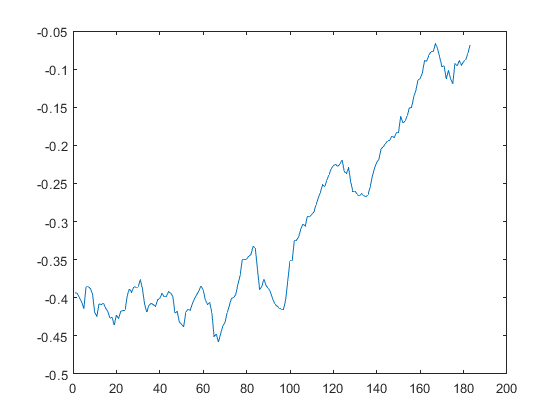
  1. The smoothed variables (purely linear model). For example labor_wedge=1-oo_.SmoothedVariables.tau_l. Like all wedges in this approach are estimated using linear decision rules.
  2. Using linear decision rules to first get log_z_t, tau_l_t, tau_x_t, and then use nonlinear decision rules to get Z_t and Tau_l_t. But investment tax is not recovered using nonlinear decision rule. So I guess all wedges are not purely linear in this approach, for example, Labor_wedge = (1-Tau_l_t) is not purely linear but investment wedge (Investment_wedge = 1./(1+tau_x_t)) is purely linear. Sorry for abusing terms, but I hope you get the idea.

Of course similar results (for example, from plotting Labor_wedge (in 2.) and labor_wedge (in 1.)) after estimation, but not exactly the same. Which one is preferred?
Labor_wedge
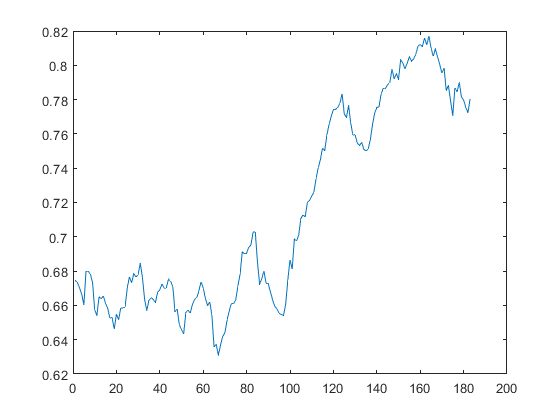
SmoothedVariables.log_labor_wedge

I am not sure what you mean. There is a large difference between the two series. One of them seems to be the log.

Sorry for the confusion. Here is what I mean, stated differently.

  1. Non purely linear model: CKM uses the linearized model only to extract the investment wedge and the decision rules. All other wedges are computed based on the original nonlinear model equations. For this purpose, the capital stock is initialized at the steady-state value in the first period and then iterated forwards.
  2. Purely linear model: This mod-file also shows how to use the Kalman smoother to directly extract the smoothed wedges. As these are based on the linearized model, they differ from the ones derived from the nonlinear equations due to Jensen’s Inequality.

My question: Yes, they differ due to Jensen’s Inequality, but both approaches are ok? And your intent was only to show that results from Purely linear model (i.e., extracting wedges directly) \approx results from Non purely linear model (i.e., extracting wedges indirectly)? Or maybe extracting wedges directly using Kalman smoother is better?

Yes, that was the intention. After entering the nonlinear model in Dynare, working with the purely linear model is straightforward and does not involve any additional steps as the smoother will provide the desired output. In contrast, using the nonlinear model to back out some of the other wedges involves tedious work and does often not make much of a difference.

Perhaps there is one drawback to using the smoothed wedges in Dynare. For example, predicting the endogenous variables using them.

Here is what I mean. If I have an explicit linear solution for the decision rules as shown below (in the form Wedges = f(data, m)), where m = (capital stock, steady-state values, decision rule coefficients) are known and f is linear. I can predict the data using m and the Wedges.

How to do that if I estimated the wedges directly? Sorry for asking a different question but it is on the same mod file.

%%%%%linear solution
% ii) compute efficiency wedge from production function
log_z_t      = z_ss+(log_y_t_data-log_y_ss-theta*(log_k_t-log_k_ss))/(1-theta)-(log_l_t_data-log_l_ss);
% iii) compute labor wedge from FOC
tau_l_t    = tau_l_ss+(1-tau_l_ss)*((log_y_t_data-log_y_ss)-(log_c_t-log_c_ss)-1/(1-exp(log_l_ss))*(log_l_t_data-log_l_ss));
% iv) use linear observation equation that relates investment x to states (x=f(tau_l,k,z,g)) to solve for tau_l 
tau_x_t = ((log_x_t_data-log_x_ss)-x_k_reaction*(log_k_t-log_k_ss)-x_eps_z_reaction*(log_z_t-z_ss)-x_eps_tau_l_reaction*(tau_l_t-tau_l_ss)-x_eps_g_reaction*(log_g_t_data-log_g_ss))/x_eps_tau_x_reaction+tau_x_ss;

Again, in the linear model, the smoother will automatically compute all that.

Hi Prof. Pfeifer, may I kindly ask where the automatically predicted output is stored? Or how to get them using the smoothed wedges?

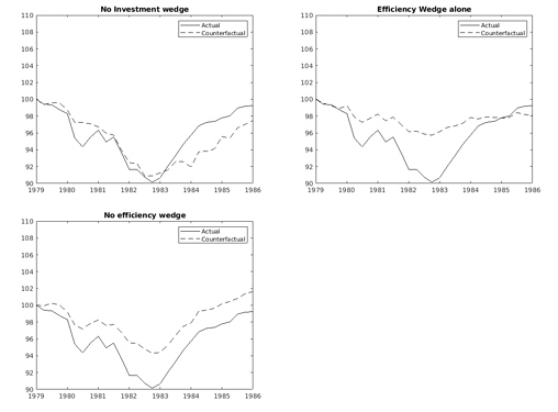
I have been able to do that manually (shown in the plots below) using the non-smoothed wedges…but I have not yet figured it out how the smoother does that automatically as you mentioned in your previous answer. Any comment on how to do that automatically using the smoothed wedges? Thanks.

Essentially you need to run a counterfactual using simult_. See e.g. Counterfactual simulations based on smoothed shocks

Thanks, Prof. Pfeifer. I realized there is one problem with using simult_ for this type of counterfactual though.

Thus, in y_=simult_(y0,dr,ex_,iorder), we simulate the model given the path for the exogenous variables (oo_.SmoothedShocks) and the decision rules.

But in the counterfactuals in Chari_et_al_2007, we need to simulate the model given the paths for the wedges (oo_.SmoothedVariables) and decision rules.

For example, given the structure of the stochastic process S_t = P_0 + P S_{t-1} + e_t where S_t = [z_t, g_t, \tau_{lt}, \tau_{xt}]), I want to, say, fix z_t = \bar{z} and simulate the model with S_t = [ \bar{z}, g_t, \tau_{lt}, \tau_{xt}].

If I understand, y_=simult_(y0,dr,ex_,iorder) simulates the model with ex_ = e_t = [e^z_t, e^g_t, e^{\tau l}_{t}, e^{\tau x}_{t}]. If I fix e^z_t = \bar{e^z}, for example, that is not the same as fixing z_t = \bar{z}.

Can simult_ be used to simulate the model given the paths for S_t = [ \bar{z}, g_t, \tau_{lt}, \tau_{xt}] (i.e., oo_.SmoothedVariables) and not e_t = [e^z_t, e^g_t, e^{\tau l}_{t}, e^{\tau x}_{t}] (i.e., oo_.SmoothedShocks)?

Or I need to make some modifications, or perhaps there is another function for it?

Which exact computation are you referring to? Generally, agents know the coefficients in the process for S_t and will react to it. So normally the simulation should work via the shocks.

Yes, agents know the coefficients in the process S_t = [z_{t}, \tau_{l t}, \tau_{x t}, g_{t}]' below.

\begin{array}{l} \begin{array}{c} z_{t}=P 0_{-} z_{-} b a r+r h o_{-} z z z_{t-1}+r h o_{-} z l \tau_{l_{t}-1}+r h o_{-} z x \tau_{x_{t}-1}+r h o_{-1} z g g_{t-1}+\varepsilon_{t}^{z} \\ \tau_{l t}=P 0_{-} t a u_{-} l_{-} b a r+z_{t-1} r h o_{-} l z+\tau_{l t-1} r h o_{-} l l+\tau_{x t-1} r h o_{-} l x+g_{t-1} r h o_{-} l g+\varepsilon_{t}^{\tau_{t}} \\ \tau_{x t}=P 0_{-} t a u_{-} x_{-} b a r+z_{t-1} r h o_{-} x z+\tau_{l t-1} r h o_{-} x l+\tau_{x t-1} r h o_{-} x x+g_{t-1} r h o_{-} x g+\varepsilon^{\tau_{x}} t \end{array}\\ g_{t}=P 0_{-} g_{-1} b a r+z_{t-1} r h o_{-} g z+\tau_{l t-1} r h o_{-} g l+\tau_{x t-1} r h o_{-} g x+g_{t-1} r h o g g+\varepsilon_{t}^{g} \end{array}

My question was that simul_t computes counterfactuals for endogenous variables (in var; block) using oo_.SmoothedShocks.

In BCA, we rather wanna set some elements of S_t = [z_{t}, \tau_{l t}, \tau_{x t}, g_{t}]' (which also belongs to var; block) to a constant and simulate the model. For example we wanna set oo_.SmoothedVariables.tau_l = \tau_{l t} = constant. And we can do that via the shocks? I don’t see how that is possible yet…using simul_t

That is indeed not possible, because it corresponds to a different model than the one run originally.