CES consumption function with durables – treatment of relative demand and prices

[AlecVanBoven]

Hi everyone,

I have a more general question about working with CES consumption functions in New Keynesian models.

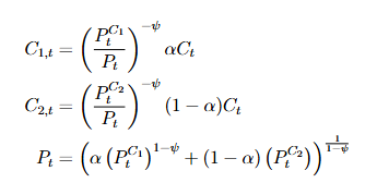
Suppose you have a CES consumption function of the kind underneath, where both goods are flow goods.

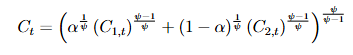
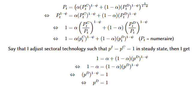
In my understanding, one would then set up the Lagrangian and solve the intertemporal optimization problem with respect to , while also solving an intratemporal allocation problem to obtain the relative demand schedules for and , as well as the price index of the CES bundle (as shown underneath).

This has always worked out fine for me.

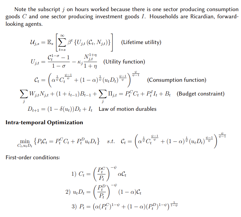
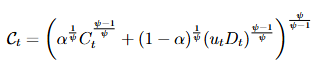
However, I get confused when durables enter the consumption aggregate.
Say the consumption function now takes the following form, where are nondurable goods (flow goods), and are services from durables, with denoting utilization.

It’s not entirely clear to me how this problem changes.

Some specific questions:

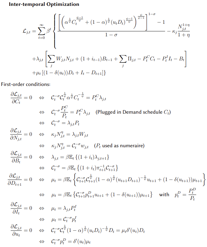
1. What is the price of ? I suppose it is not equal to the price of investing in durable goods, say . Rather, it might be ? Or should the relevant price be derived using the multiplier on the accumulation constraint for durables?

2. Should we still derive the intratemporal allocation problem to obtain relative demand schedules, or is it sufficient to simply solve the Lagrangian directly?
   In my current setup, I defined variables and as the derivatives of utility with respect to and , respectively.
   I then solved the Lagrangian and substituted in these expressions where needed.
   Consequently, I do not have explicit relative demand schedules for and , nor a derived price index of the CES consumption bundle.
   I simply define inflation as a weighted average of consumption and durable good inflation.

As a sidenote, the model with durables runs fine and behaves reasonably.
However, to provide some context for my doubt: I have a small open economy, two-sector NK model (where both durables and consumption goods are domestically produced).
When I introduce a negative discretionary income effect after an energy price shock, GDP actually increases, even though domestic consumption falls.
This happens because exports rise disproportionately.
I suspect this might be related to how I treat prices and inflation—if relative prices move too much, exports may react excessively (though other mechanisms could contribute as well).

It doesn’t feel right to continue with this specification until I fully understand whether this CES setup and treatment of prices are conceptually sound.

Any thoughts or references would be very much appreciated!

Best regards,
Alec

[jpfeifer]

You should write down the full problem setup, including the relevant budget constraints. They will contain the definition of the relevant prices. When you then compute the intratemporal first order conditions, you will obtain the correct versions of the demand equations and relative price definitions.

[AlecVanBoven]

Hi Johannes,

Thank you for your reply! I’ve outlined a simplified version of the problem and solved it according to what I think is the correct approach. The pictures below show my solution. Do you think this is okay?

Some additional questions to this:

1. What equations should be taken in the mod.file from the intra-temporal optimization problem? I always take the 3 first-order conditions in the model equations. Then I usually get confused about whether or not I need the CES function as an equation in the mod.file or not, and also whether I should take the expenditure equation (P_t \mathcal{C}_t = P_t^C C_t + P_t^D u_t D_t) in the mod.file. I have seen models where either one, or both, of these equations are added to the mod.file, but I’ve seen models where neither are added.

2. Usually I adjust technology to let relative prices = 1 in steady state (I manually calculate the steady state). Here this seems a little more complicated, and that’s also a reason why I am in doubt whether my approach is correct;
   Say that I adjust sectoral technology such that prices set by firms (p^C and p^I) are one in steady state. That implies automatically that p^D = 1 in steady state (see picture underneath).

   
   
   However, when manually calculating the SS (of the equations I’ve derived above) I find that p^D = (i + \delta)p^I, which is inconsistent with p^D = 1. I could work around this by adjusting technology such that only p^I = 1, and let p^C be free to take on a value given p^D. Nevertheless, it seemed like a red flag a bit so I wanted to ask it just to make sure.

Thanks in advance for your help!

Kind regards,
Alec Van Boven

[jpfeifer]

1. Often that equation is redundant as it is implied the price index definitions often included in the model.
2. Yes, that is indeed a red flag. It seems you cannot normalize the relative prices unless there a is an appropriate constant that allows doing that. What you describe fits this exact problem.

[AlecVanBoven]

Hi Johannes,

Thanks for getting back to me!

1. That makes sense, thanks. I can sleep on both ears now that this is not an issue.
2. Would you say it is fine to have, as I mentioned, p_I normalized to one in steady state, and let p_C endogenously take on a value based on this normalization? This is what I am trying now, but I am (2 weeks later) still very skeptical.
   If instead the way forward is to have all relative prices = 1 in steady state, do you have a suggestion on how I can use a constant to do this?

Kind regards, Alec

[jpfeifer]

2. Yes, that looks correct. You can typically normalize one price and then need to compute the rest based on this normalization. It you want all relative prices equal to 1, you often need to scale TFP in the sectors accordingly.

[AlecVanBoven]

Thanks a lot for helping!