Hi,
I have done the Bayesian estimation of a medium scale DSGE model through Dynare and the results with the respective bayesian impulse response functions are attached. Please guide me if these make some economic sense. The thing which I wanted to see was the impact of fiscal shocks on output Y and debt/gdp ration b. I will be grateful for the valuable insight on the results.estimation outcome.pdf (1023.5 KB)
1 Like
There is nothing immediately suspicious, but you did not provide anything regarding the properties of the MCMC and the mode-finding like mode_check-plots, trace_plots and stuff like that.
Dear Professor,
Thank you so much for the guidance, I have attached the mode_check-plots, trace_plot of the parameter in which we are interested and variance decomposition of the variable (debt/gdp ratio) which is the point of focus in the study. please find the attachment and guide about the areas which need adjustments. I will be grateful for the guidance.model outcome.pdf (662.3 KB)
- Some parameters seem not to be identified, i.e. there is a horizontal likelihood.
- You seem to be using too few draws
- It seems your observation equations are wrong. Your smoothed variable features a constant that should not be there.
Dear Professor,
Thank you so much for the guidance. I think the problem is with these equations. I will be grateful for help in this regard.
nr = kp(-1) + u + rk -w;
// (11) Regular labour demand;
ns = kp(-1) + u + rk - w0;
// (12) irregular labour demand;
n = etanrnr0_n0 + (1-eta)nsns0_n0; % here eta=0.80 share of regular labour force in economy
// (13) labour demand;
nr0 = 0.3335;
ns0 = 0.0700; % computed on the sample mean of labour force and multiplying it with the share of this type of force in the economy.
k0 = 0.32kp0 + 0.10kg0; % capital at steady state to get the steady state value of labour share in the economy kp=private capital, kg=public capital both have same depriciation rate.
Without context, it is impossible to know where these equations appear and what they mean. But generally, having fixed numbers appear is unusual.
Dear Professor,
Thank you so much for the direction, these equation are in the production/firms segment of the DSGE model and the steady state values are sample means and they are in the steady state block of the same model. I have attached my data file and mod file for the reference. please find the attachment and I am grateful for guidance, help and your time.bayest1.zip (85.1 KB)
- I still think you are not handling parameter dependence correctly. You should use model-local variables.
- Looking at the data series, I think I spot a seasonal pattern. You need to make sure your data is seasonally adjusted.
Dear Professor,
Thank you so much for the guidance, I will adjust the seasonal effect in the data series. And I will be grateful if you can share some example for specification of model-local variable in the DSGE models.
Dear Professor,
Thank you so much for your kind guidance, time and help. I will study the suggested information package and try to improve these aspects of the model. Have a great time.
Dear Professor,
I did the Bayesian estimation of a small open economy model with investment-specific technology shocks. I attach herewith the estimation output.
Estimation output.pdf (2.2 MB)
Please take a look at the results and guide me if something is not in order.
FYI, I have used demeaned series. I ain’t sure whether the observation equations are correctly defined (see the attached file) and don’t understand how to perform Geweke convergence test.
I have also inserted here the mod file for your reference.
TFP_IST_trend2_est.mod (9.2 KB)
Thanks and regards
Saidul
From the PDF you posted, there is nothing immediately suspicious.
Thank you so much, Professor! One quick question: is it a standard practice to report Bayesian IRFs of non-stationary variables in addition to those of stationary variables?
What matters is if a variable is of interest, not whether it is stationary.
Thanks. The responses of detrended and non-detrended variables to a particular shock are different. For example, following are the responses of detrended variables to the shocks to trend IST
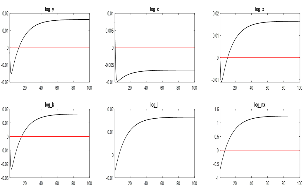
and here are the responses of non-detrended variables to the same shock:
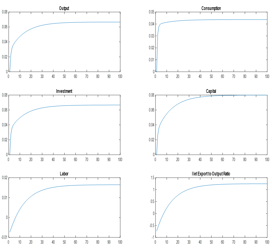
Clearly the former responses are different from the latter. In such case, which responses should I explain in the paper?
Best,
Saidul
- Why seem all IRFs permanent, including the ones of the detrended variables?
- Again, it depends on the point you want to make in your paper.
As always, I appreciate your kind response.
- I am not sure why all IRFs look permanent. Even, I don’t know how should IRFs look like as I am quite new in this literature. So, any guide would be of much help.
- Okay, I will work further on it.
May I ask you a question related to observation equation of trade balance to output ratio?
I want to add observation equation of trade balance to output ratio. I am following your code for GPU(2010). In line 167, you defined trade balance as
log(tb)= d - d(+1)*g/r;
What is the purpose of writing “log” in the left hand side? I don’t see any definition for “tb”.
Instead, couldn’t we define it as
tb= d - d(+1)*g/r;
as you defined net export to output in the code for Aguiar and Gopinath (2007)?
My definition for net export to output ratio is similar to that.
nx = ( b-q*exp(ga)^(1/(1-alpha))*exp(gv)^(alpha/(1-alpha))*b(+1) )/y;
One more thing;
In lines 232 and 242, there are two different steady state relationships for “tb”. Would you please give some clarifications on those?
Thanks!
- It’s hard to tell where the unit root comes from. Often it’s a mistake that causes permanent price level changes to spill over into the real economy.
- The reason is to counteract the
loglinear-option in the file. By definingTB=log(tb), we have thattb=exp(TB). When Dynare takes the log of all variables later on, the exp and the log will cancel. - The two definitions have to do with the log. The first definition is the level of TB, which is used for other steady state computations. The last line then takes the log of the level as the mod-file requires this.
Hi Prof. Pfeifer,
Well understood! You are making our lives easy.
One final question: I did log-linearize the model by hand and then stoch-simuled it. I found the steady-state value zeros for all model variables. To compare the solution (policy and transition functions) I ran the non-linear model with “loglinear” option of the dynare. Unfortunately, the solutions are not identical.
So, my question is: should the solutions of log-linearized model (by hand) and non-linear model with dynare’s loglinear be identical?
FYI, The purpose of log-linearization by hand is to make sure that I derived the equilibrium conditions correctly by comparing with the solutions resulted from dynare loglinear command. I also do further analysis with the linear model.
The log-linearized (hand) mod file is available here
TFP_IST_trend2_loglinear_hand.log (4.8 KB)
and the non-linear version is here
TFP_IST_trend2_loglinear_dyn.mod (4.7 KB)
My apology for asking you so many questions.