Basic question about wording in the paper

I have a basic question about wording in the paper. I am attempting to replicate Eggertsson et al. (2019). I just have one question about this paper.

I am still puzzled by Equation (59) and (60). My situation is utility functional form for real money balance (\Omega) was not given in the paper. On the footnote 40 (p.55, Eggertsson et al. 2019), it says that “households do not hold money in the numerical experiment.” What exactly does this mean? Is it safe to assume m^{b}_{t} = 0 for all t and ignore Equation (59) and (60)? or Do I assume \Omega(m^{b}_{t}) = \phi log(m_{t}^{b}) and set \phi = 0 in the dynare? or Do I not assume any functional form for utility for real money balance? If I do not assume any functional form, how can I solve for m^{b}?
I have attached Eggertsson et al. (2019) as well. Any help would be greatly appreciated. Thank you.


EggertssonJuelsrudSummersWold2019NBERw25416 (7) - Copy.pdf (1.7 MB)

They did not implement the non-linear version of the model. If you look at the log-linearized equilibrium equations, there are no m^b_t and m^s_t. I think you should write the log-linearized solution in dynare instead - equation 83 to 95.

1 Like

Dear Kofiemma,

Thank you for the response. I think you are right that they used the log linearized equations to output IRFs. I am also curious to know whether they included m^s_{t} and m^b_{t} in non-linear equations to calculate steady state values of C^s_{t} and C^b_{t}.

Sincerely,

Eric

The steady state for real variables should not depend on the money stocks. It should only depend on the real interest rate.

equation 78 and 80 are steady state values…m^b shows up there, so yeah they included it, I think. Read steady-state part. Maybe spend a little more time to go through the paper again.

Dear Kofiemma,

This is rather a strange paper. You are right about equation (78) and (80) but how can I figure out the optimal relationship between m^{b}_{t} and C^{b}_{t} if I am not given \Omega. I have been stuck on this problem for few months now. I have not gotten replies from the original authors.

Sincerely,

Eric

What I am saying is: typically, money is residually determined in these model with a cashless limit. Given the interest rate, the real allocations typically follow and from this you can compute the money stock. Here, it seems similar, but the nonlinear system is before the cashless limit has been taken. So you would need to take the limit first.

1 Like

Dear Professor Pfeifer,

Thank you for the response! m_{t}^{b} is a real money balance in this paper’s model and take part in the equation (58) (a.k.a budget constraint of borrower).

Sincerely,

Eric

Dear Professor Pfeifer

Thank you! This is a helpful response. I will search about what it means to be taking the limit.

Sincerely,

Eric

See Woodford (1998): Doing without Money: Controlling Inflation in a Post-Monetary World at https://www.sciencedirect.com/science/article/abs/pii/S1094202597900065

Steady state equations are optimal relationships without the effect of shocks (thus zero shock) in the model. They are from FOC, so they are optimal. if you hold money, then you can not consume it, so consumption falls as it says in equation 78. Not sure what optimal relationship you are referring to though.

1 Like

Dear Professor Pfeifer,

I have one question because I am struggling a lot currently. I did take a look at the paper that was provided by you.

Before I start, again to explain my situation, I am given functional form for U where U(C^{s}) is 1-e^{-qC^{s}} but I am not given functional form for \Omega.

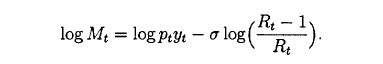
Okay, Page 37 of Woodford (1998) has following equation:

image

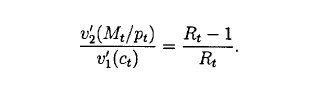
which seem to turn into following equation.

image

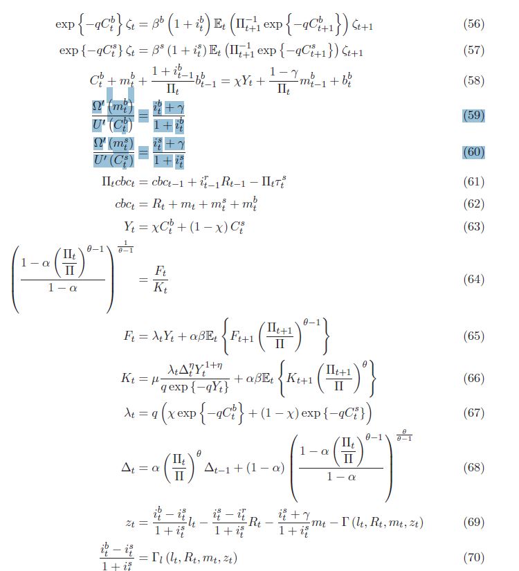
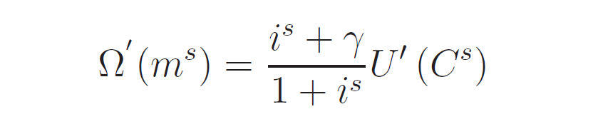
Now if I go back to Eggertsson et al. (2019),

I have following equation:

Following Woodford (1998), I converted the Eggertsson et al (2019)'s relationship between marginal utility for real money balance and marginal utility for consumption into:

C_{t}^{b} = (\frac{i^{b} + \gamma}{1+i^{b}})^{2.75} m^{b}_{t}

where \gamma is a money storage cost, m_{t}^{b} is real money balance of a borrower, C_{t}^{b} is consumption of borrower, i^{b}_{t} is lending rate, 2.75 is IES value.

I solved for steady state values for C_{t} and m^{b}_{t} but the differences in values seem to be very minor compared to values derived when ignoring money completely. That is, differences between derived steady state values for C^{b}_{t} and m^{b}_{t} (In this case, m^{b}_{t} would be 0) using Equation (56)-(58), Equation (61)-(70) and for Equation (58) using

C_{t}^{b}+\frac{1+i_{t-1}^{b}}{\Pi _{t}}b_{t-1}^{b}=\chi Y_{t}+b_{t}^{b}

and derived steady state values for C^{b}_{t} and m^{b}_{t} using Equation (56)-(58), Equation (61)-(70) along with

C_{t}^{b} = (\frac{i^{b} + \gamma}{1+i^{b}})^{2.75} m^{b}_{t}
C_{t}^{s} = (\frac{i^{s} + \gamma}{1+i^{s}})^{2.75} m^{s}_{t}

are very minor.

My question is, Did I correctly followed the procedure to derive the steady state values of variables in Cashless limit economy? If not, Could you please elaborate what it means to be taking the limit? For which nonlinear equation in Eggertsson et al. (2019) do I have take the limit? An example would be great…if possible. If not, I understand.

Sorry for the long question, Professor.

Have a great day,

Sincerely,

Eric

I think you are complicating things a little bit. In the paper you posted, they are imposing a cashless limit on the household problem, but only after deriving the non-linear equilibrium equations of the model with cash. Thus they used the objective function: \sum \beta^t [U(C_t) + \Omega(\frac{M_t}{P_t}) - V(N_t)] for the household problem of the model with cash (pages 50-52). And they used the objective function \sum \beta^t [U(C_t) - V(N_t)] for the household problem of the “cashless limit model” that they have log-linearized on pages 53,54. They did not show the steady-state equations for the “cashless limit model” because it is a simplified version of their original model (with cash)

Taking the limit as used by Prof. Pfeifer here is not taking the limit of some equation, I think. It is imposing an assumption that the fraction of households that hold money is zero. Equivalently
\Omega(\frac{M_t}{P_t}) = \phi log (m^j_t), \phi = 0 as you said before. But functional form does not matter here since \phi = 0, that is why maybe the paper has no functional form for \Omega().

So yeah, to derive the steady-state values of the log-linearised cashless limit model (pages 53-54), use the objective function, \sum \beta^t [U(C^j_t) - V(N^j_t)], and resolve the household problem.

Don’t solve the household problem with the objective function, \sum \beta^t [U(C_t) + \Omega(\frac{M_t}{P_t}) - V(N_t)] and specify that \phi = 0 for a cashless model in dynare. Maybe you can in this particular case, as \Omega' does not appear in the denumerator of any of the equilibrium equations for the model as any number divided by 0 is undefined which can cause problems in dynare. But m^j_t will still be in the other equilibrium equations of the household problem which you do not want. So yeah, use \sum \beta^t [U(C^j_t) - V(N^j_t)] for cashless model.

1 Like

Dear Kofiemma,

Thank you for the response! I have currently used your approach.

Sincerely,

Eric

But note that \phi is negligible (approaches 0) in the cashless limit theory and not exactly 0. But we can not do that numerically, so \phi = 0 is just a numerical approximation to help solve the model by ignoring money in the household problem.