I want to calibrate my model using GMM/SMM, and I’m computing second moments from real data, but some problems have arose. How I’ve proceeded: 1) downloaded raw relevant time series (most having strong seasonal component); 2) deseasonalized the time series with X-13ARIMA-SEATS (didn’t control for any particular setting, just computed deseasonalized series from basic function); 3) converted deseasonalized non-rate series (e.g. not interests nor employment/unemployment rates) to logs; 4) Extracted cyclical component using two-sided HP filter with \lambda=1600 since my data is quarterly; 5) Computed Pearson correlation matrix between all series. From here only I’m only using the cycle component from the previous process, after all this I end up with 56 obs. Then some of my problems/doubts:
-
Some of the correlations I’m getting are at odds with other papers that compute similar statistics (worth mentioning that those use a bit older data, ~8 years of difference), nevertheless some results seems really implausible, e.g. positive correlation of real M1, M2 and M3 with the nominal interest, or negative correlation between GDP and CPI with positive between GDP and inflation of CPI, or positive corr. between GDP, interest rates, and inflation.
-
Also I’d like to compute standard deviation in percent of variables, how should I calculate it? Since I thought it was another name for the coefficient of variation, but the problem is that since I’m working with the cycle the mean will be ~0, then for example computing sd(X_{cycle})/mean(X_{cycle}) gives me really big numbers (e.g. -4.484304e+16), which differ from most common statistics reported in papers (in a range between roughly ~0 and ~3).
I’ve tried to be as rigorous as possible working with the data, but not sure if I’m mistaken in some of the procedure I followed, then I’d be very grateful if you may give me some clue if I’m doing it right or where should I check again, and also some advice in how to do the computations for GMM/SMM real data second moments and checking if those’re “correct”.
Thanks!
PD: Maybe if helpful, for example applying HP as described above to aggregate household consumption, gives me a cycle that looks like this:
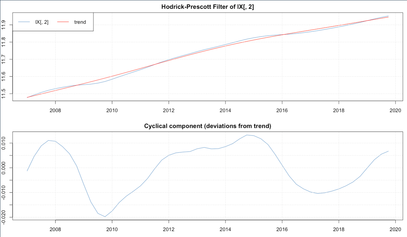
which seems like “too smooth” for me, and each cycle lasts very long (?), is that normal? Also noted that after the seasonal adjustment the data got a bit too smooth, nonetheless using data source’s seasonally adjusted data gives me very similar cycle but much more noisy.