Dear Dynare forum,
I would like to ask, whether somebody could share with me a link to some lecture notes, that provides derivation of simple three equations New Keynesian model in full nonlinear form. Thanks in advance!
Best,
Honza
Dear Dynare forum,
I would like to ask, whether somebody could share with me a link to some lecture notes, that provides derivation of simple three equations New Keynesian model in full nonlinear form. Thanks in advance!
Best,
Honza
I would recommend Gali’s textbook together with https://github.com/JohannesPfeifer/DSGE_mod/blob/master/Gali_2015/Derivation_Recursive_Pricing_Equation.pdf
Thank your very much!
Dear Prof. Pfeifer,
I am trying to implement a very basic NKE in its nonlinear form because ultimately I would like to conduct welfare analysis. Unluckily, I am getting stuck at the very beginning when I try to include the price dispersion equations set. Although I did it before reading your very detailed derivation of Gali’s chapter 3, I still don’t know where I am getting it wrong.
I have solved the SS version of the model analytically and everything seems to be fine. However, I don’t manage to meet the BK condition. I have tried two alternative approaches:
I have also tried the MODEL_DIAGNOSTICS command: It says that the Jacobian is singular. However, I don’t see where I have the unit root. Is there a way to find out which is the “redundant” equation creating problems? So far it lists 5 colinear variables and 6 colinear.
I am attaching my derivation notes so you can see how I arrived at the equations:
NKE_Baseline.pdf (180.3 KB)
Thanks in advance!
UPDATE:
Now, I am even more confused. I have slightly modified the model to drop one equation, the resource constraint C+I=Y, by putting it implicitly within the rest of equations. It still solves the SS with the same values as before but now the error message says that there are 6 eigenvalues larger than 1 in modulus for 6 forward-looking variables and that the rank condition is not verified. I am really puzzled. M02_NKE_NonLinear4.mod (2.8 KB)
Where is the Taylor rule in your model?
Good question…back to paper and pencil
Thanks!
It works!!! I can only say God bless you.
I was so much paying attention to the pricing equations that I completely overlooked this…I added a standard Taylor rule and dropped the production function (since I can derive Y without using it).
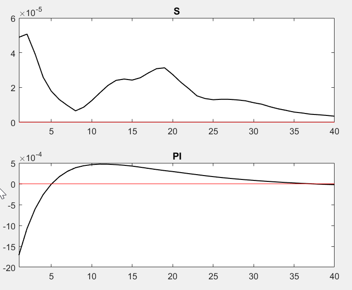
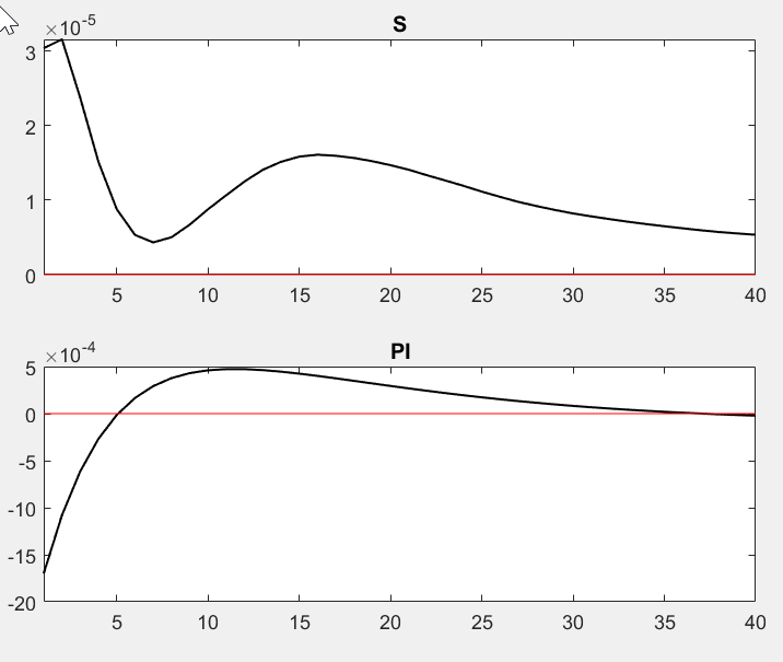
Although I get a nice IRF for inflation (PI), the line for price dispersion (S) seems to be a bit weird. Does it look plausible to you? Do you have a reference where I could learn more how to interpret these results?
Price dispersion is zero up to order=1. At order=2, you really need a lot of replications to get anything smooth.
It looks I could not go a lot further without getting stuck again. I have tried to extend the model by including a government sector that has 2 policy instruments: government consumption G (which is part of aggregate demand) and taxes on consumption and private investment (with a tax rate tauC).
At first, I was really happy because I thought I made it work. However, when I was cleaning the code, I realized that I had a typo in the Taylor rule. It originally read:
RB/RBss=S_M((RB(-1)/RB)^gammaRB)(((PI/PIss)^gammaPI)((Y/Yss)^gammaY))^(1-gammaRB);*
But it should have been (at least this is what makes sense to me since it is a deviation from SS):
RB/RBss=S_M((RB(-1)/RBss)^gammaRB)(((PI/PIss)^gammaPI)((Y/Yss)^gammaY))^(1-gammaRB);*
Where the suffix ss denotes the steady-state value.
To my surprise, when I fixed the typo it stopped to work because the BK conditions are not met. I don’t really know what is wrong. I have more eigenvalues larger than one than forward-looking variables (8 vs 7) so I understand that there is an infinite number of solutions. However, both the misspecified and the right Taylor equations have RB and RB(-1) included (they just are raised to a different exponent).
Should I try proposing a different type of Taylor rule? Something not multiplicative?
I am attaching the code, the rule that works is in line 122, and the version that does not work in line 124 (commented).
M02_NKE_G_NonLinear.mod (5.1 KB)
Thanks!
That is indeed strange. Have you compared you model setup to other standard implementations like https://github.com/JohannesPfeifer/DSGE_mod/blob/master/Gali_2015/Gali_2015_chapter_3_nonlinear.mod
Hi,
I have a question regarding adding the stickiness into a DSGE model. In the nonlinear Calvo’s approach, we usually add the following equations (Based on the Gali_2015_chapter_3_nonlinear.mod file):
[name='LOM prices, eq. (7)']
1=theta*Pi^(epsilon-1)+(1-theta)*(Pi_star)^(1-epsilon);
[name='LOM price dispersion']
S=(1-theta)*Pi_star^(-epsilon/(1-alppha))+theta*Pi^(epsilon/(1-alppha))*S(-1);
[name='FOC price setting']
Pi_star^(1+epsilon*(alppha/(1-alppha)))=x_aux_1/x_aux_2*(1-tau)*epsilon/(epsilon-1);
[name='Auxiliary price setting recursion 1']
x_aux_1=Z*C^(-siggma)*Y*MC+betta*theta*Pi(+1)^(epsilon+alppha*epsilon/(1-alppha))*x_aux_1(+1);
[name='Auxiliary price setting recursion 2']
x_aux_2=Z*C^(-siggma)*Y+betta*theta*Pi(+1)^(epsilon-1)*x_aux_2(+1);
From the first equation, we can get Pi; from the second one, S; from the third one, Pi_star and equation 4 and 5 give us x_aux_1 and x_aux_2, correct?
We also add a Taylor’s rule as follows:
 [name='Monetary Policy Rule, p. 26 bottom/eq. (22)']
R=1/betta*Pi^phi_pi*(Y/steady_state(Y))^phi_y*exp(nu);
These six equations (and six endogenous variables) in different forms and notations should be added if we want to have the Calvo’s price setting, right?
My main question is, we have the Euler equation or other equation related to R (such as R=1/Q;) that pins down R but the the Taylor’s rule also gives us R. Having these two equations does not make any problem? In fact we have 7 equations (including the Euler one or R=1/Q) and 6 endogenous variables(Pi,S, Pi_star, x_aux_1,x_aux_2 and R ). Is it correct? When a shock happens (nu), it affects R from the Taylor’s rule. How does this shock propagate through the other equations?
Thank you so much for your time
That’s not entirely right. It’s inflation and the nominal interest rate that links the Euler equation and the Taylor rule. The equations you mention above are from the firm’s pricing problem. They also determine marginal costs MC.
Thank you so much for your reply.
So which equation pins down the nominal interest rate and the inflation?
My understanding is that the Euler equation and the following one are determining R and Pi, isn’t that correct?
1=theta*Pi^(epsilon-1)+(1-theta)*(Pi_star)^(1-epsilon);
For MC, we have another equation as follows and we can get MC from that equation:
    [name='Definition marginal cost']
    MC=W_real/((1-alppha)*Y/N*S);
So what is the role of the Taylor role? What variable does it pin down? I am asking this question because Dynare says I have one extra equation considering the number of the endogenous variables and my concern is that both the Euler equation and the Taylor rule are determining R and that why I get that error message because before adding these equations, everything looks OK.
There is not a one-to-one mapping between equations and variables. Before adding which equations?
Thanks for your reply.
So as I understood, you are saying those equations can pin down MC, right? We can get MC from the FOCs of the firm’s problem (the demand for the labour) but if I understand correctly, there is no need to have that as the 5 mentioned equations can determine MC as well.