I am studying the effect of shocks to the inflation rate target on the economy (output, inflation, and interest rate) in a perfect foresight model. The impulse responses from the old steady state to the new steady state are asymmetric. Thus, raising or reducing the inflation rate target by 1% does not have a symmetric effect on the endogenous variables. Below, I show an example for output.
The asymmetricity here seems to be model-dependent because if I change some parameters, for example, the nature of the asymmetricity changes. Is there a known literature or paper on the asymmetry of shocks to the inflation target in DSGE models…to guide me on why it is occurring in my model and its economic significance? I have searched google, but nothing yet so far. I will keep searching but maybe someone knows something about this…Thanks!!
All our models are generally asymmetric if they are nonlinear. In stochastic models, people often work with linearized models. Here, the effect is less obvious. Without knowing more about the model, it’s impossible to tell what the sources of nonlinearity are in your model.
Hi Prof. Pfeifer, may I ask a related question? I have read a couple of papers on disinflationary shocks in an SVAR model, and the authors often identify disinflationary shocks using the following conditions:
A disinflationary shock has a permanent effect on the inflation rate and nominal interest rate, and other nominal variables in the long run.
A disinflationary shock has no effect on real output (and real variables in general) in the long run.
And then, they impose some long-run restrictions on the SVAR model to get the above conditions to be satisfied.
And then, they say a disinflationary shock in a DSGE model is consistent with these conditions. Is that really the case? In the plot in my earlier question, it seems nominal output did not change that much in terms of magnitude after the disinflationary shock. And it seems real output (Y-PI) would change by a similar margin/magnitude as the change in the inflation rate.
So I am confused why they identify disinflationary shock in the SVAR model using condition 2 above. Maybe, something else must also be satisfied in the DSGE model for condition 2 above to hold, yeah? THANKS.
I can’t speak to your model above. But most DSGE models feature monetary superneutrality. Changes in money growth/inflation do not affect real variables in the long-run.
Upon further checks of the papers, it seems it depends on how one defines the inflation target and how the disinflationary shock is specified.
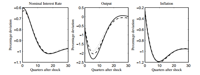
In PATRICK FÈVE, JULIEN MATHERON, AND JEAN-GUILLAUME SAHUC, they define the inflation target as follows; \pi_t^* = \pi_{t-1}^* + \sigma e_t^*, where the central bank policy rule is a function of several variables including the target \pi_t^*. Here, an unexpected decrease in e_t^* is interpreted as a disinflationary shock or a shock to the inflation rate target. It produces these IRFs (which seems to be a return to steady-state). Y-axis is labeled percentage deviation…I guess from old steady-state.
In Andrea De Michelis and Matteo Iacoviello, the target (z_t = f(\pi_t^*, e_t)) is defined as a function of two exogenous processes: \pi_t^* and e_t (both follows AR(1) process). So IRFs are similar to the one above. Thus, output response is humped-shaped after a shock to the target, and it returns to steady-state.
These two are consistent with your statement:
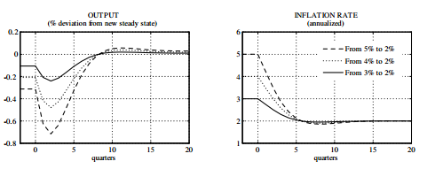
However, my model is a perfect foresight model, and I simulate it from an old steady-state (\pi_{old}^*, y_{old}, r_{old}...) to a new steady-state (\pi_{new}^*, y_{new}, r_{new}...) using initial and endval.\pi_{old}^* is the old inflation target, and \pi_{new}^* is the new target (similar to Guido Ascari and Tiziano Ropele). These are their IRFs;
The inflation rate plot on the right is from old steady-state to new steady-state. On the left (for output), however, they plot % deviation from the new steady-state. Not sure why they do this…but in my example (the graph I posted earlier), I am plotting output from old steady state to new steady-state. That is why there is a permanent change in output.
In all the papers I have listed, they call the change in the inflation target a disinflationary shock. But it seems there are two types of disinflationary shock which I did not realize before.
Thus, monetary superneutrality only applies when we are considering, say, deviations from a single steady state following a shock to the inflation rate target (which can either be a permanent or transitory shock). It seems the conditions I listed before that people use to identify disinflationary shocks in an SVAR model are based on this case. And not the case where we simulate a disinflationary shock from old to new steady-state (like in my model).
I still don’t get it. How do you break superneutrality? By giving up full indexing? That would explain the result. Otherwise, the old and the new steady state for real output should be identical.
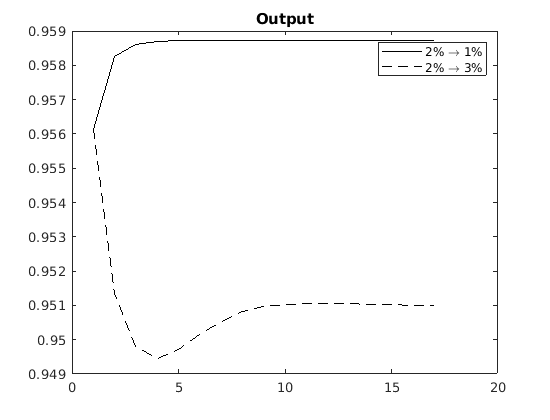
I think I get it. The plot I showed in my original question is actually for real output. Maybe that is why changing the inflation target does not change steady-state output that much.
That is, at a 2% inflation target, real output is about 0.956; at a 3% target, it is about 0.951; and at a 1% target, it is about 0.959.
I guess your point is 0.956, 0.951, and 0.959 are identical, yeah? Like, the three steady-states will not be exactly the same, but identical (i.e., a low discrepancy between them), right? Thanks!
Oh I see. By incomplete indexing, you mean something like, say \pi_t = \omega \pi_{t-1}? That is, current inflation is indexed to past inflation in the model, but only partially (with \omega<1)? If I may ask, incomplete indexing of which variable may cause that? The inflation rate, you mean?
No, I mean complete indexing in steady state. For example, consider Rotemberg adjustment costs of the form \phi/2(\pi_t-\bar \pi)^2. If you don’t make sure the \bar \pi moves with the change in the inflation target, you will have trend inflation and therefore first order effects.
Did you mean to say, “If you don’t make sure the \bar{ \pi} moves with the change in the inflation rate…”? Because \bar{ \pi} is already the target, yeah? And thus, your reply sounds like, “if you don’t make sure the target moves with a change in the target…”
So what I have in my model is something like this. Everything is the same in the initial and endval sections, except target and steady-state inflation rate (inflation_rate). The model is non-linear.
var Y C ...;

varexo target;

parameters alpha beta ...;

model;

initval;
target = exp(0.08/4);
inflation_rate = exp(0.08/4);
Y  = some expression;
C = some expression;

endval;
target = exp(0.04/4);
inflation_rate = exp(0.04/4);
Y  = some expression;
C = some expression;
Y,C here are real variables. I will investigate why the discrepancy occurs in my model. But can you confirm this statement (to make sure I understand correctly)…
“Even in a non-linear model, a non-zero inflation rate has no effect on real variables in steady-state unless there is some sort of incomplete indexation in the model.”
The last statement is true in most models. There must be something that breaks long-run non-neutrality. The main exception is the literature on trend inflation around Guido Ascari’s work. Here, there is no indexing.
No \bar \pi is a parameter set by researchers. Most often it refers to the inflation target and will change with it. But you could have the target \pi^* change without \bar \pi changing. That would result in imperfect indexing.
But one more question, if I may ask. So here, \pi^* is sort of an implicit inflation target in the model, yeah?
And you are right, \bar{\pi} (which is the steady state inflation rate in my model) is set by me, though under the varexo block (so technically, maybe not a parameter:)). I see some papers calling it the inflation target. So I call it the inflation target in my model.
But in your reply, you refer to \pi^* as target. Do you mean the implicit inflation target? Which can then change without \bar{\pi} (the explicit target) changing?
And I guess your previous reply was that I should make sure \pi^* moves with \bar{\pi}. How can I do that. Like define \pi^* in the model, and then do \pi^* = \bar{\pi}?
Thanks a lot. Maybe I can ignore the small change in steady-state real output when I change the explicit inflation target in my model, and consider Y_{ss} = 0.956, 0.951,0.959 to be identical.
This statement explains the lack of full indexing in my model, right?
Something fundamental like imperfect indexing? Thus, the explicit inflation target changing without the implicit target changing? Are there ways one can remove imperfect indexing?