Hi,I am reading replication code for leeper (2017)and hope to get some help with the dreivation.
Rhoss = (1 - (1/AD))*(1/bet);
gammss = gamm100/100;
expgss = exp(gammss);
Rss = expgss/bet; // real or nominal interest rate since pi = 1 in steady state
Rbarss = (Rss - 1)*100;
Pbss = 1/(Rss - Rhoss);
AD is average duration,gammss is growth rate .Does anyone know how the price of bond pb is derived?
KLss = (wss/Rkss)alph/(1-alph);
OmegLss = (KLss^alph) - Rkss(KLss) - wss;
y - ((yss+Omegss)/yss)alphk -((yss+Omegss)/yss)*(1-alph)*l=0;
The production function is of usual cobb-douglus type.Does anyone understand omegl here?Why doesn‘t TFP enter the linerized production fuction?Is it detrended?
Yes,the dynare code in the link is the same as that on mbb model base.I have posted there as well but there are only very few users ,who are not very active.Besides ,I thought the question is more about the theory,so I posted and hoped to get some help here. Enclosed is the dynareUS_LTW17_rep.mod (29.2 KB) code.
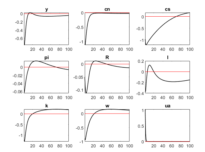
Hi.I am running stochastic simulation of the model now.But the result is quite counterintuitive.A positive productivity shock would be contractionary in the model.Is it natural or reasonable?Thanks.
If y is the level of output und the productivity shock is temporary, then no. If it is a shock to the growth rate of productivity and y is detrended output, then yes.
As in the replication code I am studying,real variables are detrended using the stable growth rate of productivity .And productivity shock is in exponential form .But the result of a productivity shock is quite counter-intuitive .
I have checked the paper you referred to,which is relevant and inspiring. But I think the utility function in that paper is quite uncommon in recent literature and it does not capture many effects or factors .And,returning to the irf drawn using Leeper’s code with shock to trend,I still think it would not be very reasonable that consumption,investment and ouput of US all plunge suddenly .
You are still not grasping the issue here. If there is a permanent shock to TFP and you have a detrended model, then the IRF will be relative to the trend. On impact, the trend will immediately jump up, showing a relative decline. That would look very much different if you add back the trend as in the mod-file I linked.
But I still have some doubt.If variables are detrended log-linearized as Y hat=(Y-Yss)/Yss as in Leeper’s and Y and Yss have the same trend ,the sign of impluse response should be the same,whether you add back the trend or not and therefore the graph I posted would still look strange.If you use dlog(y) instead of log(y) in your replication code,I think the result could be different.
You are still missing that Yss changes. Again, see
//Now back out IRF of non-stationary model variables by adding trend growth back

log_Gamma_0=0; //Initialize Level of Technology at t=0;
log_Gamma(1,1)=g_eps_g(1,1)+log_Gamma_0; //Level of Tech. after shock in period 1

// reaccumulate the non-stationary level series; note that AG2007 detrend with X_t-1, thus the technology level in the loop is shifted by 1 period
for ii=2:options_.irf
    log_Gamma(ii,1)=g_eps_g(ii,1)+log_Gamma(ii-1,1);
    log_y_nonstationary(ii,1)=log_y_eps_g(ii,1)+log_Gamma(ii-1,1);
    log_c_nonstationary(ii,1)=log_c_eps_g(ii,1)+log_Gamma(ii-1,1);
    log_i_nonstationary(ii,1)=log_i_eps_g(ii,1)+log_Gamma(ii-1,1);
end

//Make the plot
figure('Name','IRF of non-detrended variables to a trend productivity shock');
subplot(3,1,1)
plot(1:options_.irf,log_y_nonstationary)
title('Output')
subplot(3,1,2)
plot(1:options_.irf,log_c_nonstationary)
title('Consumption')
subplot(3,1,3)
plot(1:options_.irf,log_i_nonstationary)
title('Investment')
From what I understand of your code,y is detrended but not log-linearized as percentage deviation of the steady state,as you are writing in the non-linear form.Adding log_gamma back to log(y)only serves to add back the trend but if it is compared with its steady state level Yss ,which grows at the same rate as the trend,the graph and result would look different.
The point here is that there are shocks to the trend, so the Yss will change immediately. An IRF in deviations from the new steady state (which Dynare shows) will look very differently from one in deviation from the old steady state (which you seem to expect).
But I suppose they should be the same when output has already been first detrended and then log-linearized?If ouput is log-linearized as percentage deviation from the steady state,does it matter if it is detrended or not ,since it is just dividing both the numerator and denominator by the same trend?