Hello everyone,
Very happy to join this forum ![]()
The paper can be found here:
I’m reading this paper, because there seem to be two ways to calculate the welfare; one is the Linear-Quadratic (LQ) approach, and the other is the perturbation method. But after searching in this forum, Dynare now still has some limitations to completely solve out the welfare. See
(If my understanding was wrong, please kindly point out, thx!)
Then looking backward to LQ, I found Benigno and Woodford (2005JEEA and 2012JET) are highly cited literature. The paper 2012JET is a bit abstruse to me. Yet Benigno and Woodford mentioned Sutherland 2002 partially parallels their methodology in a simple way. This is the underlying reason I come here.
~ ~ ~ ~ ~
My specific question, however, is pertinent with matrix manipulations ![]()
(I emailed Sutherland, and got no reply. Perhaps it’s too trivial?)
One of the key steps is illustrated around equation (23) on page 7:
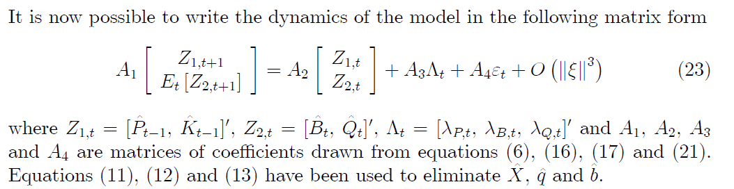
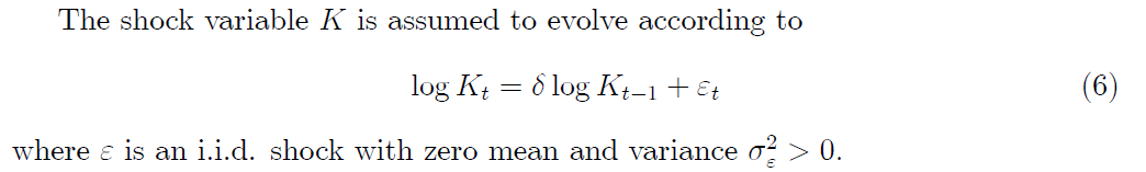
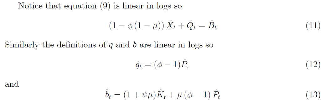
To facilitate the discussion, I snapshoot these equations again:
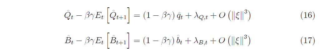
together with
Now we can rewrite them as follows, ignoring terms of \mathcal{O}(||\xi||^2):
\hat{P}_t = \gamma \hat{P}_{t-1} + \left[\frac{1-\gamma}{1-\phi(1-\mu)}\right](\hat{B}_t-\hat{Q}_t)+\lambda_{Pt},
\hat{K}_t=\delta\hat{K}_{t-1}+\varepsilon_t,
\beta\gamma\mathbb{E}_t[\hat{B}_{t+1}] = \hat{B}_t-(1-\beta\gamma)(1+\psi\mu)\hat{K}_t-(1-\beta\gamma)\mu(\phi-1)\hat{P}_t-\lambda_{Bt},
\beta\gamma\mathbb{E}_t[\hat{Q}_{t+1}] = \hat{Q}_t-(1-\beta\gamma)(\phi-1)\hat{P}_t-\lambda_{Qt}
and then into the matrix form, just like equation (23):
A_1\left[\begin{array}{c}
\left[\begin{array}{c}
\hat{P}_t \\
\hat{K}_t \\
\end{array}\right]\\
\mathbb{E}_t
\left[\begin{array}{c}
\hat{B}_{t+1} \\
\hat{Q}_{t+1} \\
\end{array}\right]\\
\end{array}\right]
=A_2
\left[\begin{array}{c}
\left[\begin{array}{c}
\hat{P}_{t-1}\\
\hat{K}_{t-1} \\
\end{array}\right]\\
\left[\begin{array}{c}
\hat{B}_{t} \\
\hat{Q}_{t} \\
\end{array}\right]\\
\end{array}\right]
+A_3
\left[\begin{array}{c}
\lambda_{Pt}\\
\lambda_{Bt}\\
\lambda_{Qt}
\end{array}\right]
+A_4\varepsilon_t
where
A_1=
\left[
\begin{array}{cc|cc}
1 & 0 & 0 & 0 \\
0 & 1 & 0 & 0 \\
\hline
(1-\beta\gamma)\mu(\phi-1) & (1-\beta\gamma)(1+\psi\mu) & \beta\gamma & 0 \\
(1-\beta\gamma)(\phi-1) & 0 & 0 & \beta\gamma
\end{array}
\right]
A_2= \left[ \begin{array}{cc|cc} \gamma & 0 & \frac{1-\gamma}{1-\phi(1-\mu)} & \frac{1-\gamma}{1-\phi(1-\mu)} \\ 0 & \delta & 0 & 0 \\ \hline 0 & 0 & 1& 0 \\ 0 & 0 & 0 & 1 \end{array} \right], A_3= \left[ \begin{array}{ccc} 1 & 0 & 0 \\ 0 & 0 & 0 \\ 0 & -1 & 0 \\ 0 & 0 & -1 \end{array} \right], A_4= \left[ \begin{array}{c} 0 \\ 1 \\ 0 \\ 0 \end{array} \right]
At the current stage, A_3 is not important, as said in equation (25):
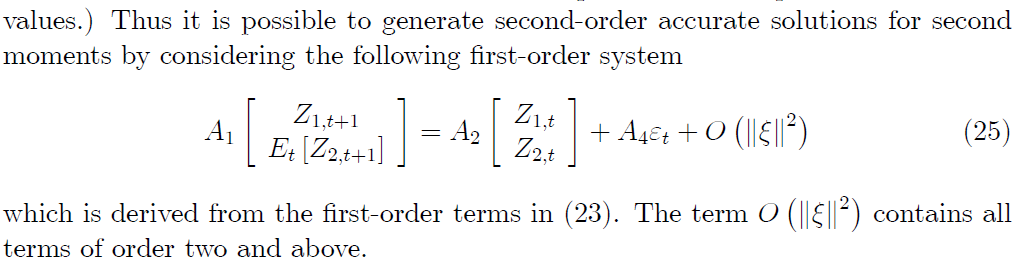
On page 14, the author continues that:

How to transform A_1, A_2 into matrices G and F?
Especially, by partitioning A_2, the sub-matrix A_2(1,2) is singular ![]()
(Footnote 11 on page 8 hints (44) and (45) directly come from (23)-(25))
Sooo sorry for this long question…and if my calcuation contains errors, please let me know. Thank you!