Hello, everyone
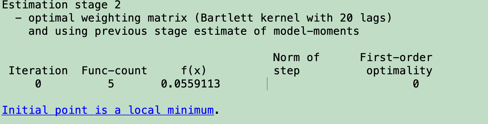
I am new to Dynare and encountered a problem with GMM estimation: the optimization completed after the first iteration in the second stage. Therefore, the estimated parameters always stay at the initial values I input, as you can see from the snapshots.
It is not shown as a bug because the program continues to run, but I cannot get any useful information from such estimation. Can anyone help me with that? I have attached the .mod file, the data file, and the steady-state computation file. Great thanks!
Best,
Mingzuo
myfile.xls (31 KB)
example3.mod (2.9 KB)
example3_steady_state_helper.m (255 Bytes)
Matlab’s optimizer performs surprisingly poor without explicit bounds set. Try e.g.
example3.mod (2.9 KB)
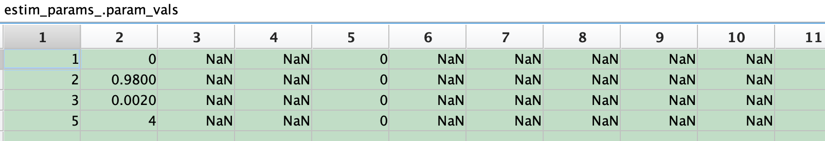
Thanks a lot, Prof. Pfeifer. It works this time! Can I ask you another question: where can I find the estimated parameters? At present, I am only able to find the parameters in my command window. However, aren’t they supposed to be found under “estim_params”? Now they are still shown as NaN there.
estim_params_ is a setup structure for internal use. Results are stored in oo_.mom. For example oo_.mom.gmm_stage_2_mode.parameters
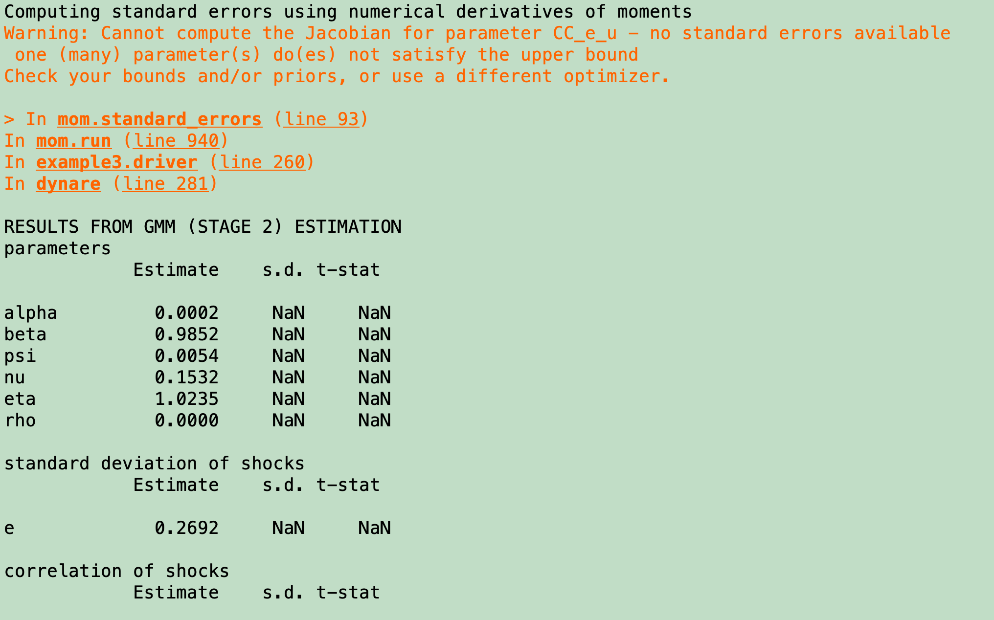
Thanks for your clarification, Professor. I have another question to follow up on: under some circumstances, the standard errors of the estimated parameters are missing, like below. Is it a big problem? In other words, can I feel safe using these estimated parameters?
You can see the warning message above. There was an issue during estimation due to a parameter hitting the upper bound. Which optimizer did you use?
I think the optimizers are all set at their defaults: options_mom.mode_compute=13 and options.mode_compute=4. Is there a way for parameters not to hit the bounds?
example3.zip (12.6 KB)
The error message is misleading. The problem is that CC_e_u hits the upper bound, preventing to compute the Jacobian using finite differences.
Hello. Prof. Pfeifer. Thanks for your reply, and I have another question. I was wondering if it would be Okay if the model is approximated at the second-order but around a deterministic steady state. I ask this question because uncertainty plays a vital role in my model relevant to portfolio choices (the reason I want to preserve the second-order term). But at the same time, I cannot compute the stochastic steady-state but the deterministic one. In this sense, can I still trust the results I get based on deterministic steady-state and second-order approximation? The current results show that the deterministic steady-state is substantially different from the theoretical moments implied by the solution.
I think an equivalent question is whether Dynare can itself find the stochastic steady-state when solving the model.
That is hard to answer. Dynare does not support computing the risky steady state. But portfolio problems are usually indeterminate at the deterministic steady state as all assets pay the risk-free rate without any risk. You need to know whether you can solve the portfolio problem with that type of setup. But from what I understand, there are techniques like the one by Devereux/Sutherland to solve such issues in Dynare.
Thanks for clarifying, Professor. My case is a little special in which the agents finance the accumulation of short-term liquidity with long-term debt. Liquidity has a direct utility like money(MIU), whereas long-term debt faces a higher return with its size due to financial frictions. Therefore, even in a deterministic case, there will be a well-defined solution (the steady-state). However, I need to have a second-order solution because liquidity has another role in redeeming long-term debt during a financial crisis due to a fire-sale of the latter. With these, do you think it works with a second-order solution around the deterministic steady-state?
That sounds like a second-order approximation around the deterministic steady state should be sufficient.
Hello, Prof. Pfeifer. Another question to bother you now. In my model, I have an unobserved shock, e, of which the standard deviation sigma_e needs to be estimated. I specify the standard deviation in two ways: in the first one, I use the conventional command “stderr e, 0.01, lb, ub”; while in the second one, I specify e=lambda*u where u follows a normal distribution with a pre-determined standard deviation, say 0.1, and my task is to estimate lambda. Mathematically, these two methods should be equivalent. However, I found they could generate quite different estimation results. I find it hard to understand the reason. Can you help me clarify it?
Do you get the same initial value of the objective function?
Hi, Professor. I am a bit confused with “the initial value of the objective function”. Do you mean the Fval obtained by the minimization routine in the first stage? Then they were different. Perhaps the answer to my question is that I did not start with the same initial values and bounds of the standard deviation of the shock under these two specifications. Am I right?
Yes, optimization is typically inherently dependent on the starting values. That should explain the difference.