I made some changes to the way Y is being read and then the file gives the following error at the end :
The variance of the forecast error remains singular until the end of the sample
My codes are as below:
data_index = cell(1, 100); % You need to replace 'smpl' with the actual number of samples

number_of_observations = 100;  % Replace 'smpl' with the actual number of samples

no_more_missing_observations = 0;  % Set as needed

load Y
Y
% Y = transpose(data_table);  % Transpose to match the required format

%Y = randn(pp, smpl);  % Replace with your actual data matrix

start = 1;  % Index of the first observation

last = 100;  % Index of the last observation

a = zeros(5, 1);  % Replace with your actual initial state vector

P = eye(5);  % Replace with your actual covariance matrix

kalman_tol = 1e-6;  % Tolerance parameter for Kalman filter

riccati_tol = 1e-6;  % Tolerance parameter for Riccati iteration

rescale_prediction_error_covariance = 1;  % Set as needed

presample = 0;  % Set as needed

T = [0.4200 0.0000 0.0000 0.0000 0.0000; 0.0350815232 0 0 -0.0000 0.0000; 1.92168733 0 0 -0.0000 0.0000; 0.0147342398 0 0 0.0000 0.0000; 0.807108677 0 0 0.0000 0.0000];  % Replace with your actual transition matrix

Q = [1.0000 0.0835274363 4.57544601 0.0350815232 1.92168733; 0.0835274363 0.00697683261 0.0382175275 0.00293026970 0.160513616; 4.57544601 0.382175275 2.09347062 0.160513616 8.79257661; 0.0350815232 0.00293026970 0.160513616 0.00123071327 0.0674157186; 1.92168733 0.160513616 8.79257661 0.0674157186 3.69288218];  % Replace with your actual covariance matrix of structural innovations % this is transition cov from python

R = [0 17.9491966 0 0 0; 0 0 0 0 0; 0 0 0 0 0; 0 0 0 0 0; 0 0 0 0 0]; % Replace with your actual mapping matrix % this is observation matrices from python

H = [1];  % Replace with your actual covariance matrix of measurement errors %this is observation covatriance

Z = 1;  % Replace with your actual vector of indices for observed variables

mm = 5;  % Replace with the actual dimension of the state vector

pp = 1;  % Replace with the actual number of observed variables

rr = 1;  % Replace with the actual number of structural innovations

Zflag = false;  % Set as needed

diffuse_periods = 0;  % Set as needed

occbin_ = [];  % Set as needed
occbin_.status = false;


% Call the function

[LIK, lik, a, P] = missing_observations_kalman_filter(data_index, number_of_observations, no_more_missing_observations, Y, start, last, a, P, kalman_tol, riccati_tol, rescale_prediction_error_covariance, presample, T, Q, R, H, Z, mm, pp, rr, Zflag, diffuse_periods, occbin_);
I will be really grateful for your help. I still haven’t been able to figure out the issue with the singularity error. If you can help - I might be mistake in declaring certain matrices or vectors may be.
Thank you for your help. I am trying to map the following model in dynare and to your matlab codes but something seems to be wrong in mapping it exactly. Requesting for help.
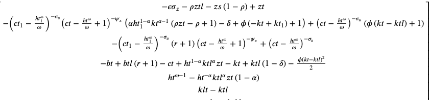
I tried to re-work with model equations to correctly map them but it still throws a few error. I am attaching the “.mod” file. I will be grateful if someone can help in letting me know what might be going wrong with the set-up. I am trying to map the following set of equations (All terms are on left-hand side so the equations appear as below:)
Carefully check your equations and their description. You did not even make clear the distinction between parameters and variables. Also, first make sure the IRFs are the same in a basic model without manually introduced auxiliary variables. Only then start manually introducing auxiliaries.
I have cross checked my equations thoroughly. My .mod file has all parameters and variables distinction now.
I read about auxiliaries on the forum and in the manual and I am still not sure how you would introduce it here - I have expectations as well as a k_t+2 term but the k_t+2 term is being replaced by a variable kl which is just set equal to k_t+1 to avoid dealing with a k term 2 periods ahead (k_t+2).
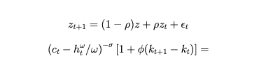
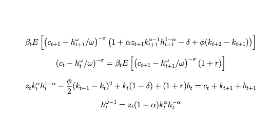
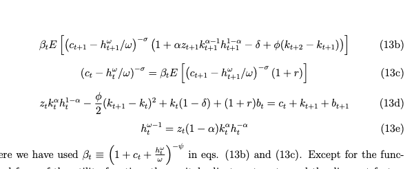
I am attaching the .mod file and below a clear set of 5 equations which I am trying to map.
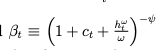
where
My variables are [z,c,k,h,b], while parameters are [delta, r, alpha, psi, rho, sigma_u (sigma in the model), sigma_z(variance attached to the shock), phi, omega] RBC_model_check (1).mod (3.0 KB)
There are still various issues, in particular the timing. The first equation cannot be correct.
You should start with a basic working version of the model and then use write_latex_dynamic_model to see how Dynare does the substitution using auxiliary variables.
Thank you Prof. Pfeifer for your help. I could figure out the problem.
I had a few general questions about model solution and bayesian estimation though:
From the literature that I have gone through so far, I see that linearization (higher order perturbation methods) are more accurate than log-linearization. Do they necessarily lead to different results - this is the problem which I might be facing in my model. Also, log-linearization throws an error of “hessian” not being positive definite, which disappears once linearization is used.
Second and third order perturbation methods will lead to some terms being linear, while others non-linear or quadratic. However, the Kalman Filter uses a set of linear equations so how do the second and third order approximations map to a simple multivariate Kalman Filter in dynare? [Do Sylvester equation solution method help in this]. Is there somewhere I can read about it to understand better?
If the model is nonlinear, different approximation orders will lead to different results, since the approximated equations will be different. If the approximated model is non linear you cannot use the kalman filter, you will need to go for a nonlinear filter (just set order to a value greater than one in the estimation command). Options for nonlinear filters are described here:
Thank you for sharing the details about approximation methods. How can we be sure that approximated model will be linear or non-linear in dynare?
Most of the models approximated end up being linear and then go through Kalman Filter but I wish to understand - is there a way to know if my approximated model is linear or not?
That’s up to you… You need to choose the approximation order when using commands estimation or stoch_simul. The default order of approximation with stoch_simul is 2, while with the estimation command the default order is 1.
Thank you Prof. Adjemian for your help and explanation.
I am trying to map the following set of equations to dynare. However, I still get the following error:
Blockquote
One of the eigenvalues is close to 0/0 (the absolute value of numerator and denominator is smaller
than 0.0000!
 If you believe that the model has a unique solution you can try to reduce the value of
 qz_zero_threshold.
Blockquote
I guess this arises due to incorrect time mapping of the model but I have checked multiple times and I am not able to figure out what might be going wrong. Below are the equations I am trying to map. I have made multiple attempts but something seems to go wrong. I am attaching the code file and below are the equations. I will be glad for your help. RBC_model_check (4).mod (2.6 KB)
Thank you Prof. Pfeifer. I am really gratefuk for your help.
I checked (13a) as you suggested and yes, it is a very simple SOE model with z being pre-determined in this case.
I has a few clarificatory questions:
Like you suggested that how should give some initial values. What determines when should I and when I should not give initial values in a model? Can I read about it some where?
I am aware that you have a summer school for a week every year. However, given my PhD commitments I cannot apply for it this year. I would like to attend it at some point though. Given this, what can be a way to have a holitic overview about Dynare?. I have been through the manual. I saw some Dynare Tutorial Videos by Willi Mutschler. Going through all of them would be good idea? Or is there some other path you suggest or any other source? I also came across some papers on dynare. What would be an organized way to gain a holistic knowledge about dynare’s functionality?
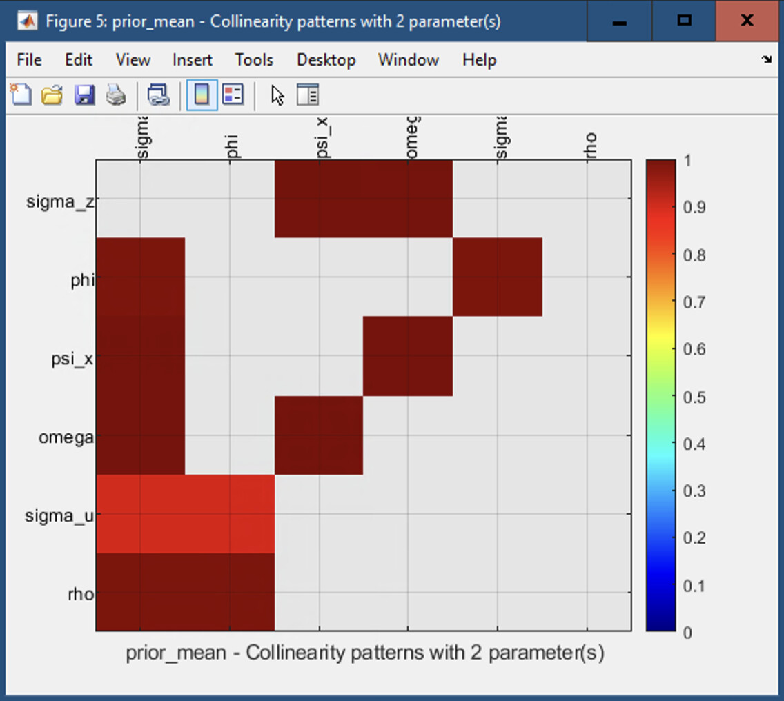
Further, having run the above model, I ran identification tests and found the following results. given my model, I want to be sure about identification issues in my model. Given below, what do you suggest? does it mean that sigma_z and sigma_u and rho are unidentified? I saw your explanation about each of diagnostics plot in manula on plots that you have but I am still struggling to understand everything. If you or someone in the forum could help.
The thing is that since my Python codes which just follow simple algorithms for bayesian estimation do not give similar results and seem to reflect identification issues, I need to dig down deeper why that is occuring? I have now checked my Python algorithms part by part with MATLAB codes - gensys, csminwel, mcmc so far and they give same results (in parts). So what I am anticipating is that it might be the methodology which might be the reason for the differences. I am mid-way checking Kalman Filter results for both taking help from your matlab codes on the website (as you suggested).
I went through the material you suggested and it was extremely helpful. I had 2 questions:
If I have my data already detrended and logged. Can I just map it as my observed variable i.e. suppose k is observed and I have already logged and detrended data. Can I write varobs as k and not log_k since I do not need to take log of ’ k’ now (as I already have done it in my csv file). And do I still declare “logdata” in my estimation command or it is not required since I am already declaring varobs as ‘k’.
Further, I know that no. of observables are equal to no. of shocks. Is it still possible or is there a way that we can have more observables than no. of shocks? Document on observation Equations mentioned that " having more shocks than observables is also not uncommon". So, can I have more observables and I can declare the standard errors of those observables as "stderr " under estimated params command?
Altough Professor Pfiefer must answer to the quesions but as I know your first question’s answer is yes as I know.
Your second euestion’s anwser is no. Maximum number of observable variables is equal to the number of shocks in the model and not more than it. Altough you can estimate your DSGE model with fewer observable variables of the shocks. For example when you have six shocks in your model you can estimate the model with six observable variables or less than six observable variables but not more than six variables.