Thank you so much!
- I reset the upper bound to 50% of std.dev of observable and estimate under following scenarios:
a) mode compute : 4 and uniform prior. This yields the following error:
“matrix must be positive definite with real diagonal”
b) Then I change the mode compute to 6 and use inverse gamma prior (also uniform prior). Both give me similar results in terms of variance decomposition. Here’s the inverse gamma version
Posterior mean variance decomposition (in percent)
           eps_al      eps_vl      eps_ga      eps_gv      eps_xi  eps_tby_ME
g_y         31.85        3.61       42.05        8.29       14.20        0.00
g_c         15.42        0.06       45.10        2.38       37.02        0.00
g_x         24.51       16.83       18.41       11.80       28.45        0.00
tby          7.66        0.91       37.52       19.81       24.24        9.86
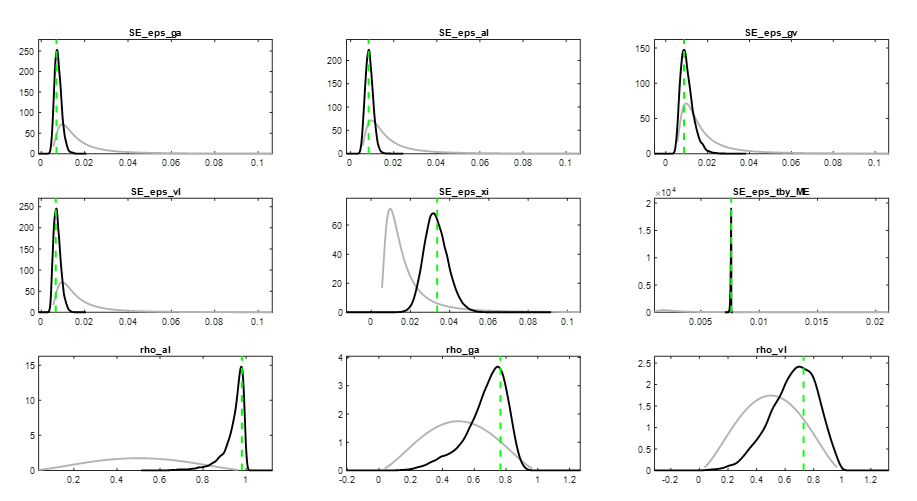
As you can see, the contribution of tby_ME comes down to less than 10%. However, the priors and posteriors for eps_tby_y look unusual.
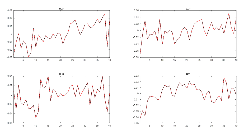
- Did you ask me to check the following plot?
Both actually observed data and smoothed series are identical. Do you want me to check somethingelse?
My original concern was the value of the the debt sensitivity of interest rate (psi) parameter. When I set it to a low value of 0.001, the contribution is trivial. However, either calibrating psi with a relatively high value (0.0355) or estimating it makes the contributions of measurement error and preference shocks to variance decomposition very high.