Policy frontier

[Ankit]

Dear Sir

Thank you for your reply. However, when I am coding these parameters in steady state model (as you did) , the dynare is giving me Waring as
%%
MODEL_DIAGNOSTICS: The Jacobian of the static model contains Inf or NaN. The problem arises from:

Derivative of Equation 15 with respect to Variable ygap (initial value of ygap: 0)
Derivative of Equation 15 with respect to Variable wgap (initial value of wgap: 0)
Derivative of Equation 40 with respect to Variable wgap (initial value of wgap: 0)
Derivative of Equation 13 with respect to Variable wigap (initial value of wigap: 0)
Derivative of Equation 14 with respect to Variable wigap (initial value of wigap: 0)
Derivative of Equation 16 with respect to Variable wigap (initial value of wigap: 0)
Derivative of Equation 20 with respect to Variable wigap (initial value of wigap: 0)
Derivative of Equation 13 with respect to Variable wegap (initial value of wegap: 0)
Derivative of Equation 14 with respect to Variable wegap (initial value of wegap: 0)
Derivative of Equation 17 with respect to Variable wegap (initial value of wegap: 0)
Derivative of Equation 20 with respect to Variable wegap (initial value of wegap: 0)
Derivative of Equation 40 with respect to Variable wegap (initial value of wegap: 0)
Derivative of Equation 15 with respect to Variable sgap (initial value of sgap: 0)
Derivative of Equation 16 with respect to Variable cigap (initial value of cigap: 0)
Derivative of Equation 17 with respect to Variable cegap (initial value of cegap: 0)
Derivative of Equation 16 with respect to Variable nigap (initial value of nigap: 0)
Derivative of Equation 38 with respect to Variable nigap (initial value of nigap: 0)
Derivative of Equation 17 with respect to Variable negap (initial value of negap: 0)
Derivative of Equation 38 with respect to Variable negap (initial value of negap: 0)

MODEL_DIAGNOSTICS: The problem most often occurs, because a variable with
MODEL_DIAGNOSTICS: exponent smaller than 1 has been initialized to 0. Taking the derivative
MODEL_DIAGNOSTICS: and evaluating it at the steady state then results in a division by 0.
MODEL_DIAGNOSTICS: If you are using model-local variables (# operator), check their values as well.
%%
No such warning is coming if I have model parameters as parameters or as local variables.
At the same time the optimal value is still not same as when I am running them individually.
Can you please help me this.

Thanks in advance.

[jpfeifer]

I would need to see the files.

[Ankit]

Thank you very much for your help Sir. I am still in bit of trouble. I am running modified mod file with steady state model block separately and one time within loop by changing the value of f.
When run separately at value of f = 0.5, the optimal value is 0.68 and 0.89.
But when run within the loop, at f=0.5, the optimal value is 0.66 and 0.96.
Is this ok to have this kind of difference ?
Is this because of some kind of optimisation problem ? I am also getting
Warning:Non-Finite fitness range.
In Cmaes at 974
In dynare _minimize_objective at 360
In Osrl at 132

I am using opt_algo=9 in my code.
I will be very helpful for comment on this.
Thanks in Advance

[jpfeifer]

Yes, that is strange and you should investigate this.

[Xuyanxia]

Hi, Prof Pfeifer, I add your above code to my mod file and I have the following error:

PP.mod (11.4 KB)

ERROR PP.driver (line 675)
var_piH(grid_iter)=oo_.var(piH_pos_var_list_,piH_pos_var_list_);

ERROR dynare (line 281)
evalin(‘base’,[fname ‘.driver’]);

Thanks.

[jpfeifer]

You are trying to read out piH, but you only requested pi as an output:

osr(opt_algo=9) ygap pi;

[Xuyanxia]

Thanks a lot ! I was careless. I modified the model and it works now.However ,I am confused about a question.In command window , there is:
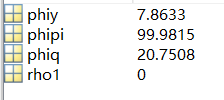
OPTIMAL VALUE OF THE PARAMETERS:

        phiy          31.7588

       phipi           38.978

        phiq          8.11791

        rho1                0

Objective function : 0.000193508
But in oo_.osr.optim_params ,there is :

Then, for my above model, which are the optimal parameters?

[jpfeifer]

That depends. You have a loop iterating over parameters at the end. The workspace will contain the results after that loop.

[Xuyanxia]

Specifically, I hope to get the following figure and table:

After I run the above model file ,I get a figure:

I think I get the same figure as above one that I uploaded earlier:

I am not sure whether I am correct. Still, I have no idea about how I can get the data in the table:for example,for every parameter weight ,the corresponding OSR parameters and variance ( used for computing loss ),etc.Where can I find them?

[jpfeifer]

You are currently doing a loop where you compute the optimal rule parameters for each weight. You simply need to extract the results from oo_.osr.optim_params at each step.

[Xuyanxia]

Thanks. Now I use OSR to compute optimal simple rule for A given value of the objective function weight. Then I change the objective function weight manually and can get what I want.
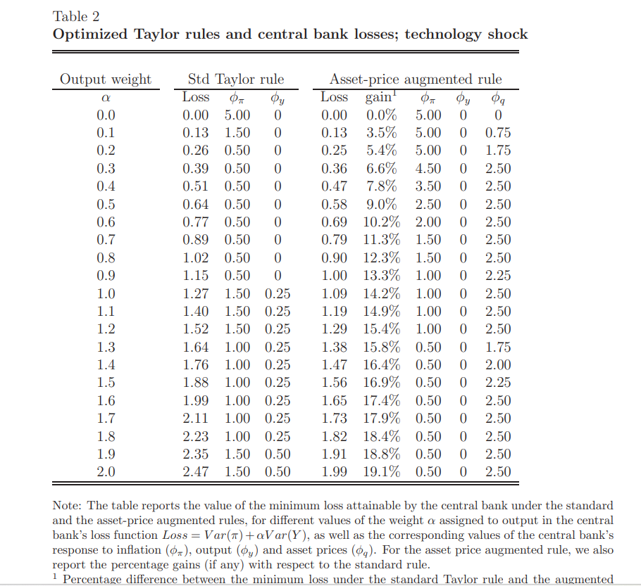
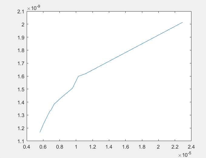
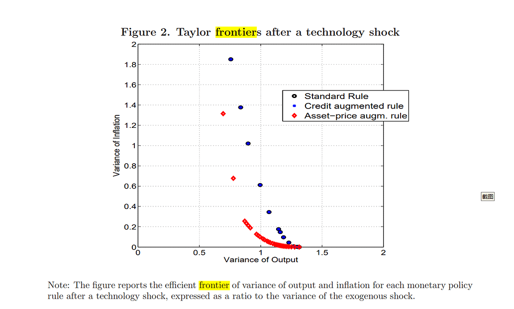
Now I have another problem:After I run my above model file, I get a curve that slopes upwards to the right . It seems strange to me, cause I haven’t seen this kind of shape for Taylor curve. So, is there something wrong with my model?

PP.mod (11.4 KB)
However ,I got a normal shape Taylor curve for the first time,like:

The only difference is that there is multiple shocks for the first time, but one shock for this time.

[jpfeifer]

With one shock, divine coincidence many hold, which would explain the figure.

[Xuyanxia]

Prof Pfeifer, How can I put two Taylor curves in a figure ,like

The optimization parameters are, osr_params phiy phipi (say, standard rule) and osr_params phiy phipi phiq rho1, respectively.
I already uploaded my mod file, see PP.mod.
Thank you for your continuous guidance and help.

[jpfeifer]

You need to run the two sets of optimization over the respective grids, save the results, and then combine the plots in Matlab. This is not a Dynare-specific issue.

[Xuyanxia]

I have the same idea, but I don’t know what to save.
About my code，can you tell me what to save?
optim_weights;
pi 1;
y 0.5;

end;
osr_params phiy phipi ;

osr_params_bounds;
phiy, 0, 5;
phipi, 1, 5;

end;

osr(opt_algo=9) y pi;

% make loop silent
options_.nofunctions=1;
options_.nocorr=1;
options_.noprint=1;
options_.irf=0;
options_.silent_optimizer=1;

options_.osr.opt_algo=9;

% find position of variables in variable_weights
y_pos=strmatch(‘y’,M_.endo_names,‘exact’);
pi_pos=strmatch(‘pi’,M_.endo_names,‘exact’);

% find position of variables in var_list_
y_pos_var_list_=strmatch(‘y’,var_list_,‘exact’);
pi_pos_var_list_=strmatch(‘pi’,var_list_,‘exact’);

weight_grid=0:0.01:1;
n_grid_points=length(weight_grid);
var_y=NaN(n_grid_points,1);
var_pi=NaN(n_grid_points,1);
for grid_iter=1:n_grid_points
M_.osr.variable_weights(pi_pos,pi_pos) = weight_grid(grid_iter);
M_.osr.variable_weights(y_pos,y_pos) = 1-weight_grid(grid_iter);
oo_.osr = osr(var_list_,M_.osr.param_names,M_.osr.variable_indices,M_.osr.variable_weights);
if oo_.osr.error_indicator==0
var_y(grid_iter)=oo_.var(y_pos_var_list_,y_pos_var_list_);
var_pi(grid_iter)=oo_.var(pi_pos_var_list_,pi_pos_var_list_);
end
end
figure
plot(var_y,var_pi)

[jpfeifer]

var_y and var_pi store the variances.

[Xuyanxia]

Thanks!