Hello another time professor, so in order to estimate my parameters following your code, the only thing i need to do is to change in run_filter_and_smoother_AR1.m the observable series (x) by my data??. If this is right, what type of data should I use to feed into the code?
Thanks in advance, I hope you can help me.
Instead of the simulated data at the beginning of the file, you need to provide some covariance stationary data with mean 0.
Thank you very much professor, I have some more doubts:
- How many variables do i have to include in my data?? I have thought in including data of the VIX index as I want to estimate the parameters of the uncertainty shock, but I do not know if I have to include more variables such as Consumption, Output, Investment, etc.
- In order to have a covariance stationary data with mean 0 I have to eliminate the trend and/or the unit roots (if they exist) and substract the mean from the series, right??
- Finally, in order to achieve 2, can I proceed differentiating my data??
- The code estimates a univariate process.
- Yes, if there is a trend, you need to eliminate it and you should express your process in deviations from the mean.
- Yes, you can use demeaned growth rates, if you want to.
- The VIX should be covariance stationary. You would only need to demean it.
I’m struggling a little bit with the code. I replace this part of the cod: observable_series=x;
by my data which contains only one column: observable_series=my_data.csv; and I get acceptance rates of 0. I do not know if I have to change more things of the code or if it is caused by the data.
Thank you very much for your time.
Please provide a plot of the data.
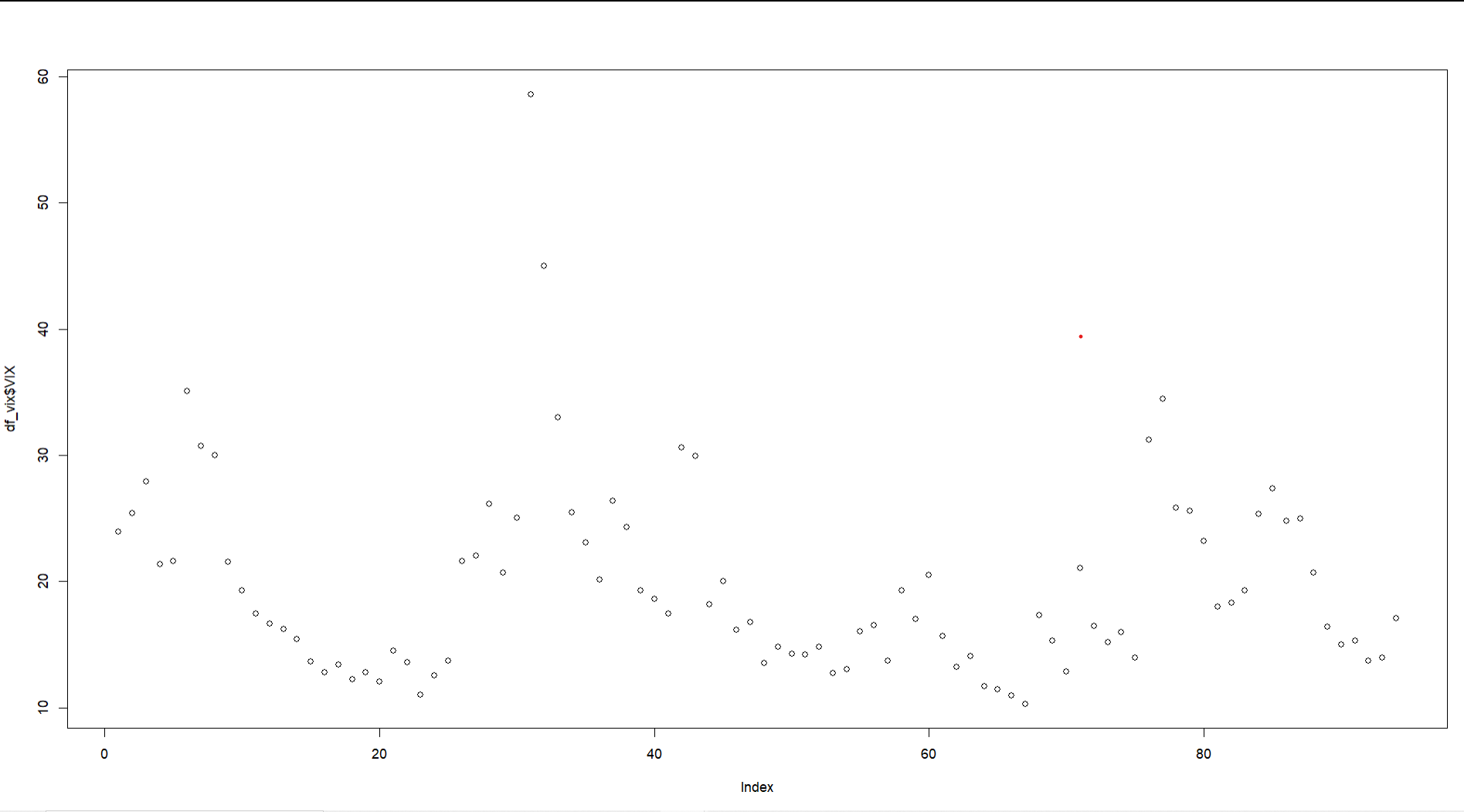
This is the data that I am using (it is basically the data from the VIX index). However i took logs and i have demean the series and now i obtain aceptance rates between 20% and 40% and parameters that are like the ones in the literature.
I wonder if it possible to obtain different values for the parameter sigma_bar. When I introduce into my model the parameter that I obtain with the current code (I obtain a sigma_bar similar to log(0.01)), the model simulates IRF counterintuitive. However when I introduce a sigma_bar of 0.01 (the value used by Leduc & Liu) i observe more plausible IRF (with precautonary saving etc.)
That sounds a lot like the data scaling and the model equations do not match.
So if i take logs of my variable and then i demean it, it would be a correct approach??. Doing that is the only way i found to run succesfully the code and obtain acceptance rates of around 40%
Yes, that conforms to the setup of my code, which used percentage deviations.
- You need to adjust periods to the length of your data.
plot(1:length(xhat_smoother),xhat_smoother,....)
- Yes, that should be correct. But you also need to adjust the lower level functions if you delete the
exp.
Thanks for your reply, Prof Pfeifer.
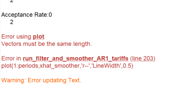
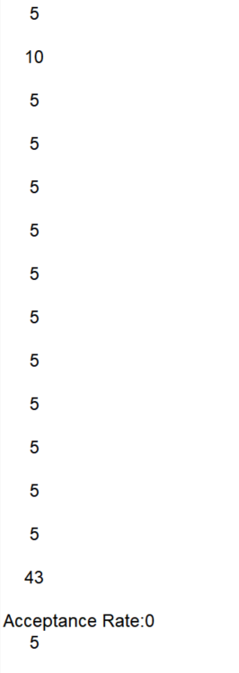
- But the first question is that the acceptance is 2, I think the data processing procedure is correct.
- What is the difference between these two setting methods:exp volatility and level volatility? Will they have different impacts on the results?
- No, the acceptance rate is 0 and there is a problem with observation 2. You need to debug the problem.
- It’s about the interpretation, i.e., whether the shock is in percent or not. Due to the difference in scale, you need to make sure you account for that in setting the parameters.
It means there is still something fundamentally wrong. You are losing all particles before you reach the end of the sample.
Thanks for your help,Prof Pfeifer.The issue has been resolved.
Hello another time Professor. I wrote here some months ago and I finally managed to run the Particle Filter. i have now a doubt because i wanted to estimate the AR with SV to obtain its parameters and introduce them into a DSGE. My problem is that i have estimated the process using data with quarterly frequency but my model is calibrated in annual frequency. I suppose that for re-scaling the autocorrelation coefficients I should raise them to the power of 4, but for the volatility of second moment and the mean I do not know how to re-scale them.
Another question that I have is why we need to use covariance stationary data to estimate the AR with SV (I have to justify this in my Master’s Final Dissertation).
I hope you can help me another time ![]()
PS: I will include your name in the acknowledgments section of my master’s thesis.
- Why do you calibrate your model to quarterly frequency? The usual procedure is to set up the model at quarterly frequency and then aggregate the model data if you need annual moments.
- Data can only be meaningfully represented as an AR process if it is covariance stationary. That is a result following from the Wold Theorem. Any covariance stationary process can be represented as an infinite order MA process. An AR process is a special form of such an infinite order MA process.
The issue is that I have used quarterly data for estimating the AR with SV because with annual data I did not have enough observations to proceed with the estimation. But my DSGE model is set in annual frequency, so my question was how to transform that parameters from the AR-SV (that are estimated with quarterly data) into annual, in order to have all parameters with anually frequency.
Thank you for your time.