Did you check whether the signs match? Is there dynamics to return debt to the non-binding regime?
- Yes, I assume that as P_N (relatives prices picks up following an interest rate shock): Firms profit increase and demand for labor increase leading to an increase in the non tradable GDP (This mechanism is clear in Nonbinding case-attached), this process continues until GDP become high enough to relax the binding constraint)
- The complementary slackness condition requires \mu_t \ (D_t +\phi*(W_t*N_t + \pi_t)) = 0.
I have implemented this in Dyane as follows:
[name=‘Borrowing Constraint eq8’, relax=‘occ’]
mu = 0;
[name=‘Borrowing Constraint eq8’, bind=‘occ’]
D = -phi*(W*N + ppi);
and then declared:
occbin_constraints;
name ‘occ’; bind D <= -phi*(W*N+ppi);
end;
If this is the right way to set up the occasionally binding constraint, then how \mu is determined when the constraint is active ?
@jpfeifer any advise please whether I am implementing occbin constraint part right in dynare ? (part 2 above) I am attaching an updating version of the code .
SuddenStopSGU_steadystate.m (4.4 KB)
SuddenStopSGU.mod (8.0 KB)
The implementation looks correct.
Thank you !
SuddenStopSGU.mod (7.5 KB)
SuddenStopSGU_steadystate.m (4.4 KB)
@jpfeifer Hi again,
I continued investigating the code, the model works fine when the borrowing constraint does not bind i.e. \phi > 1.9, but when \phi=1.9 or less, IRF graph diverges and does not revert to baseline scenario although Steady state and Bk condition all are fine. Any advise where to investigate or where I might messed up ?
One thing I have suspected I messed up with is the definition of the shocks. In Mendoza (2002), shocks process for tradable endowment is e^{\epsilon^{T}_t}, productivity shock A_t=Ae^{\epsilon^{N}_t}, and interest rate shock e^{\epsilon^{R}_t} are all Markov process. If I imposed the productivity shock as: \epsilon^{N}_t =log{Z_t}=\rho*{log(Z_{t-1})}+\epsilon_t (to allow for a productivity shock today to have an effect on tomorrow’s production too) while the other two shocks \epsilon^{T}_t and \ \epsilon^{R}_t are iid~(0,\sigma^2) then it would affect model’s return mechanism to non-binding case ?
An AR1 process is a Markov process. Your IRFs suggest that, once you enter the binding regime, the model explodes instead of converging back to the non-binding regime. You need to find out why. Have you tried just running the model for the binding regime?
Thank you prof.
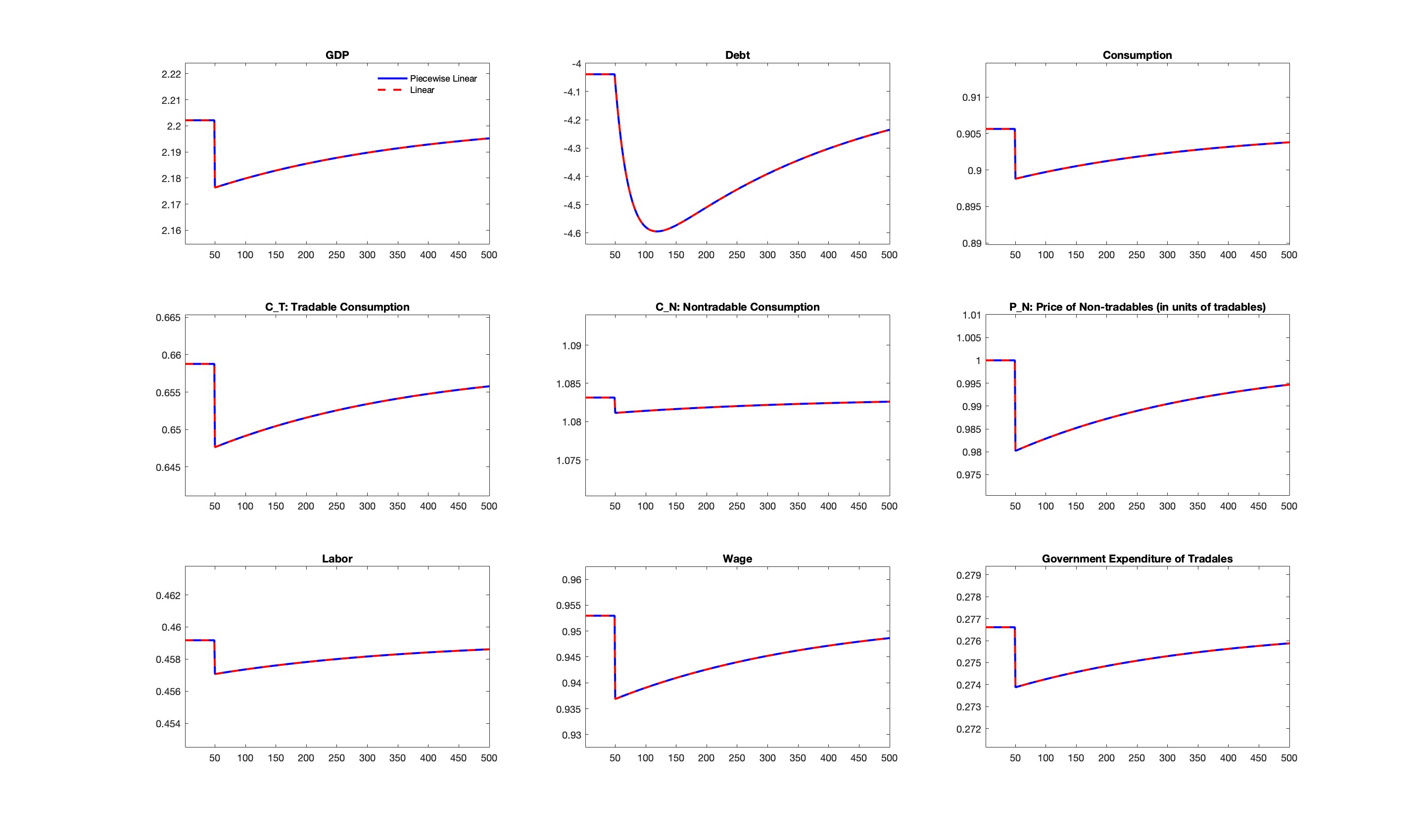
Yes and this is what is puzzling me. I have tried to run the binding scenario alone using -stoch_simul- and it behaves perfectly well and returns to its steady state. Please see the binding case results.
bind.mod (3.9 KB)
Hi Prof.,
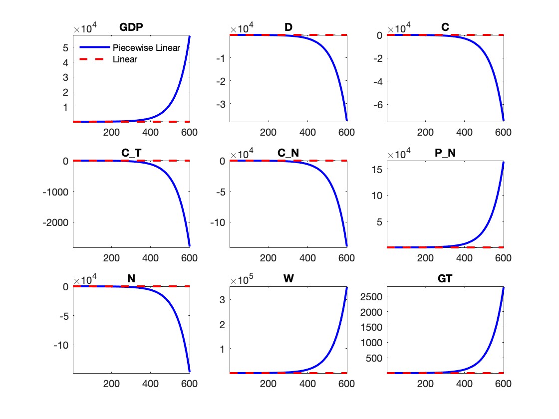
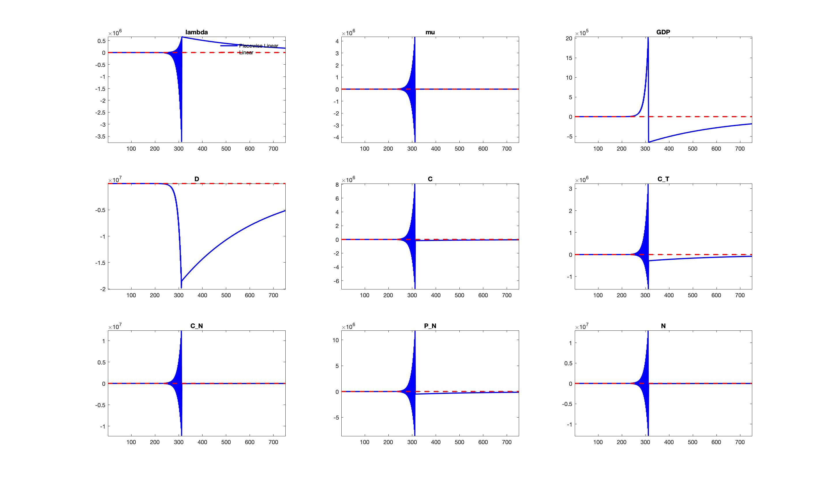
I used Mendoza’s (2002) calibration values and I I get below simulation results with ossiilating results before model converges. The BK condition is satisfied but one of the stable eigenvalues is near 1 (0.997) with no complex eigenvalues and I have doubled check the timing convention where only debt is predetermined in the model.
When the model is solved for relaxed borrowing, simulation results are reasonable and converge smoothly. Only when the binding constraint is active, then simulation results ossiliiates. Please note that the behavior of the simulation after oscillation phase is the correct for all variables except for debt.
Also whenever I amend the \delta: elasticity of labor supply then the labor supply equation becomes indeterminate (complex) .
Any advise if possible ?
SuddenStopSGU.mod (5.6 KB)
SuddenStopSGU_steadystate.m (4.4 KB)
@jpfeifer how to retrieve eigenvalues of the binding constraint ?
I don’t know the solution. There must be a problem with the binding regime. These oscillations do not make sense and the binding regime being there for more than 500 periods also looks strange.
Thank you prof., But one more thing that would help me debugging the problem and generally speaking. Given that Dynare recalculates rank condition when the binding regime prevail:
-
If the binding regime Bk condition is satisfied but one of the stable roots is negative. Then in this case, there will be oscillations despite BK being met. Does this indicate wrong model specification ?. I mean despite BK being met, should I suspect model mis-specification (generally speaking) ?
-
In other occasions, despite BK condition being met, one of the none stable roots (those who are equal to the forward looking variables) is complex. In this case ossoliations in simulation or IRF will not show up as the solution of the model is independent of these unstable roots. Right ?
What do you mean with
The bind condition can in principle violate the BK conditions as long as you return to the relax condition that must be BK stable.
Oscillations in the solution are almost always a sign of problems in the model specification (either timing or parameters).
Thank you prof.
I meant in the above that when I run the binding case separately BK condition sometimes is satisfied while one of the stable roots is negative. In this case oscillation is due to this negative eigenvalue but this does not negate the fact that there is a model specification (as you indicated in your reply) even when BK holds. Right ?
Yes, even if the BK conditions hold, that result rarely makes economic sense. But depending on the model, you may have intended oscillations. Ask the model-builder.
Many thanks Prof.