I am looking at the discrete model from Dewachter and Wouters 2014 (Endogenous risk in a DSGE model with capital-constrained financial intermediaries), who have a non-linear constraint and use third order perturbation in Dynare. And I have some problems understanding/using the pruning function correctly.
When I simulate their model using third order perturbation and no-pruning, I get good simulation results that do not show any strange behaviour. However when I then try to do a GIRF, I get a GIRF that is exploding in most variables. Now I understand that I should use pruning to prevent such explosive behaviour, but if I use pruning in my simulations, my variables are not well-behaved and have bigger range and move far away from the deterministic steady state.
Is there anything I’m missing in using pruning with third order perturbation? Is there a way to not do pruning for the simulations but do it for the GIRF?
In that case, you can use the simult_-function to generate GIRFs yourself. There you can select whether you want pruning or not. But more fundamentally, you should either work with pruning all of the time or not at all. And how can the GIRFs explode?
I am using the simult_ - function based on your RBC_state_dependent_GIRF.mod example. Here, however if I try to set options_.pruning=1; I get an error-message (which I think makes sense since I haven’t used pruning for the simulations).
Right now, my GIRFs turn very large in the sixth period after the shock (and then into NaNs), which is what I thought I could prevent with pruning. And I understand completely that I should be consistent throughout the model, but the simulations only feature the model characteristics (as documented by Dewachter and Wouters) in the unpruned setting.
Now, I do understand that pruning should help when I want to increase the shock-size/ the number of simulations. However, when I do use pruning, I am back to my problem above where the non-linearities are removed from the simulation and the GIRFs (and the simulation is more dispersed and the economic interpretation of some variables seems to be reduced (e.g. leverage in the non-pruned model ranges from 200 to 400%, but in the pruned model from -1000 to 400%)).
My question now is whether this is a wanted feature of pruning - that it removes the non-linearities and that it reduces any economic interpretation one could make?
Basu and Bundick did not really use GIRFs, they compute the IRFs at the stochastic steady state, which is a very particular conditioning set for the GIRFs.
No, pruning creates a whole bunch of problems. But we accept them to avoid explosive simulations. Note that the IRFs at the stochastic steady state should be a lot more stable than normal GIRFs, so you could work without pruning even for larger shocks. Also not that you do not need several simulations as there is nothing to integrate out. One simulation suffices.
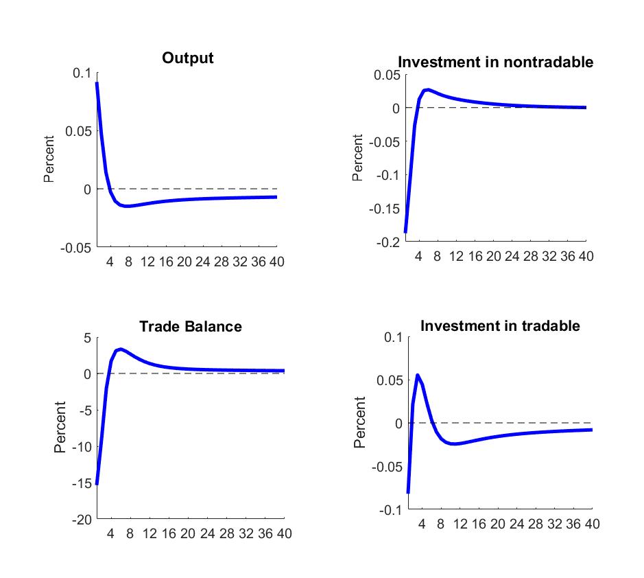
In my work with two production sectors and small open economy, I have an uncertainty shock to the TFPs. The market clearing equation of tradable good is Y_t=C_t+IT_t+IN_t+TB_t. Where IT_t, IN_t, TB_t are the investments in two sectors and the trade balance. However, the plotted IRF is really hard to be explained. Facing the uncertainty shock, consumption and investment, as well as trade balance drop. Yet, the output goes up. Is it possible to have such a scenario?
Thanks for your reply. I work in levels with the following simulation command. stoch_simul(order=3,k_order_solver,noprint,irf=0,nofunctions)
And I have the capital adjustment cost. The model could be with nominal rigidities. And the price adjustment cost will enter the market clearing condition of output: Y_t=IT_t+IN_t+TB_t+C_t+Adj.Cost
However, the IRFs are similar to the ones presented here. In this case, do you have any suggestion on how to solve this problem?
Maybe I misunderstand your suggestion. The simulation works in level. And this GIRF is based on the stochastic steady state. And the IRF is the percentage deviated from this stochastic steady state. I borrow the following source code for the computation of GIRF.
Do you mean that this approximation method could lead to the problem I faced? If I want to check whether it is really due to this approximation method. Do you have any suggestion on other methods to get the IRF in this third-order environment.
Thanks for your suggestion. I go back to my code and check whether I use log_Y or Y. Currently, my code uses Y but not log_Y in the model part of the mode file. I attach the part of my mod file to generate the IRF.
shock_mat_with_zeros=zeros(burnin+IRF_periods,M_.exo_nbr); %shocks set to 0 to simulate without uncertainty
IRF_no_shock_mat = simult_(oo_.dr.ys,oo_.dr,shock_mat_with_zeros,options_.order)‘; %simulate series
stochastic_steady_state=IRF_no_shock_mat(1+burnin,:); % stochastic_steady_state/EMAS is any of the final points after burnin
shock_mat = zeros(burnin+IRF_periods,M_.exo_nbr);
shock_mat(1+burnin,strmatch(‘e_sigma’,M_.exo_names,‘exact’))= 1;
IRF_mat = simult_(oo_.dr.ys,oo_.dr,shock_mat,options_.order)’;
IRF_mat_percent_from_SSS = (IRF_mat(1+burnin+1:1+burnin+IRF_periods,:)-IRF_no_shock_mat(1+burnin+1:1+burnin+IRF_periods,:))./repmat(stochastic_steady_state,IRF_periods,1); %only valid for variables not yet logged