Hi all,
I made a quick and simplified version of Leeper (Dynamics of Fiscal Financing in the US); I have capital tax, labour tax, and government spending. There is no transfers and no consumption tax like in the original Leeper model.
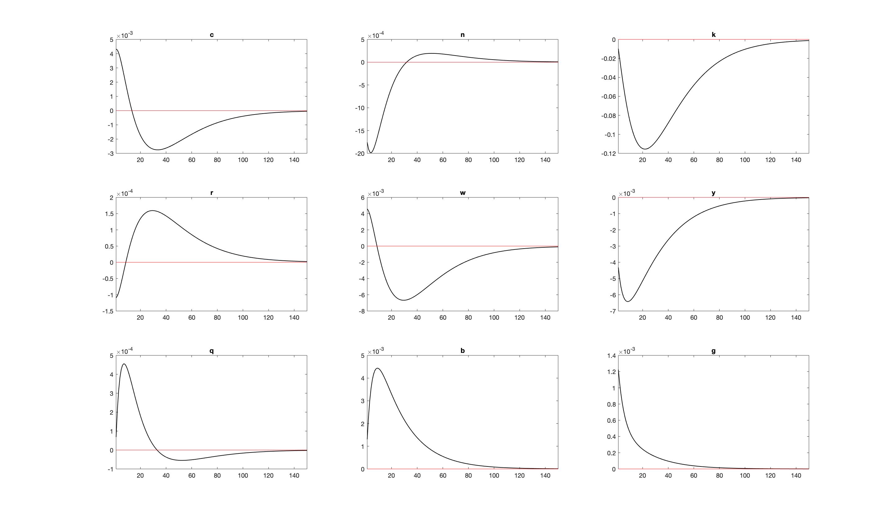
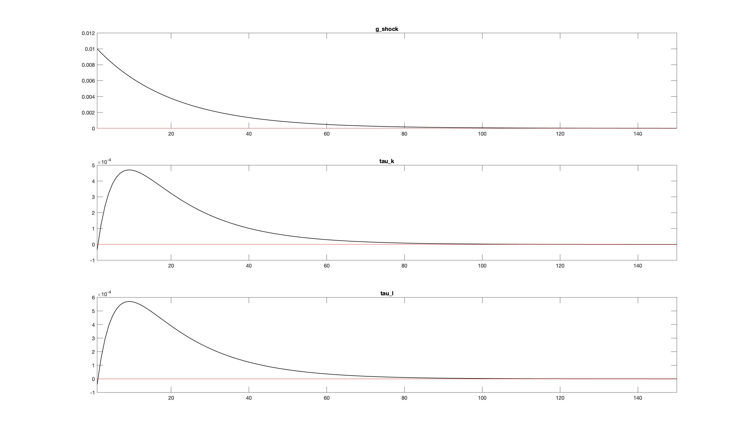
In the IRF plot, it shows that output declined with higher government spending. I am not sure why would this be the case?
The goods market which is y = c + i + g, means that if g increases, then y should increase as well. The only way that increase in g leads to decrease in y, is if investment decrease. Does this mean that household now switch from investing in capital to investing in government bonds?
Code;
var c n k z r w y q b g g_shock tau_k tau_l;
varexo e_z e_g;
parameters beta theta delta rho a psi psi_g;

beta = 0.99;
delta = 0.025;
theta = 0.36;
a = 1.72;
rho = 0.95;
psi = 0.5;
psi_g = 0.5;

params = [beta theta delta a psi];
init = [0.5 0.1 1 0.1 0.1 0.1 0.01];

options = optimset('Display','iter');
[ss,Fval,exitflag] = fsolve('rbc_gov_ss',init,options,params);

model;
// First order conditions for households.
(((1 - tau_l) * w) / c)  = a / (1 - n);
beta * ((1/c(+1)) * (1 - tau_k) * (r(+1) + 1 - delta)) = (1 / c);
beta * (1/c(+1)) = (q / c);

// Household budget constraints.
c + k + q * b = (1 - tau_l) * w * n + (1 - tau_k) * r * k(-1) + (1 - delta) * k(-1) + b(-1);

// Firm production.
y = exp(z) * k(-1)^(theta) * n^(1 - theta);
w = (1 - theta) * exp(z) * k(-1)^(theta) * n^(-theta);
r = theta * exp(z) * k(-1)^(theta - 1) * n^(1 - theta);

z = rho*(z(-1)) + e_z;

// Government budget constraint.
tau_l * w * n + tau_k * r * k(-1) + q * b = b(-1) + g;

// Government rules
//t / ((1/beta)* (0.3396*1.23358) - (0.0922*1.23358)) = - psi * log(b / (0.3396*1.23358)) - psi_g*log(y/1.23358) + t_shock;
//g / (0.0922*1.23358) = - psi * log(b / (0.3396*1.23358)) - psi_g*log(y/1.23358) + g_shock;
//tau_l / 0.223 = psi * log(b / (0.3396*1.23358)) + psi_g*log(y/1.23358);
//tau_k / 0.184 = psi * log(b / (0.3396*1.23358)) + psi_g*log(y/1.23358);
//t / (0.223 * steady_state(w) * steady_state(n) + 0.184 * steady_state(r) * steady_state(k) + steady_state(q)*steady_state(b)-0.0922*steady_state(y)-steady_state(b))  = - psi * (b / (0.3396*steady_state(y)))  - psi_g * (y/steady_state(y))  + t_shock;
g / (0.0922 * steady_state(y))  = - psi * (b / (0.3396*steady_state(y)))  - psi_g * (y/steady_state(y)) + g_shock;
tau_l / 0.223 = psi * (b / (0.3396*steady_state(y)))  + psi_g * (y/steady_state(y));
tau_k / 0.184 = psi * (b / (0.3396*steady_state(y)))  + psi_g * (y/steady_state(y));

// Gov shocks
//t_shock = rho*(t_shock(-1)) + e_t;
g_shock = rho*(g_shock(-1)) + e_g;

end;

initval;
z = 0;
c = ss(1);
n = ss(2);
k = ss(3);
r = ss(4);
w = ss(5);
y = ss(6);
q = ss(7);
b = 0.3396*1.2815;
g = 0.0922*1.2815;
//t = (1/beta)* b - g;
tau_k = 0.184;
tau_l = 0.223;
end;

model_diagnostics;
resid;
steady;

shocks;
var e_z = 0.01^2;
var e_g = 0.01^2;
//var e_t = 0.01^2;

end;

stoch_simul(periods=2000, drop=200,irf = 150,order=1);