Hi, everyone.
I’am a student to study macroeconomics.
I start to study dynare coding.
In most cases, A(productivity) = 1 or TFP follows the AR process.
But I want to reflect A_{t+1} = 1.01 * A_t.
Is it possible? How to make coding this case?
or is this meaningless?
You can just write the following in Dynare if you define “a” as productivity:
“a(+1) = 1.01*a;”
But don’t you need a shock term for “a(+1)” meaning that the process for “a” could be described by the following: “a(+1) = 1.01*a + epsilon;” where “epsilon” could be an i.i.d.?? In that case, remember to specify epsilon in the “shock frame” in the modifle.
Thanks for answering.
I tried to make code.
var A0t A2t A3t;
parameters A0_growth A_growth;
A0_growth = 1.01^10;
A_growth = 1.02^10;
model;
A0t(+1)=A0_growthA0t;
A2t(+1)=A_growthA2t;
A3t(+1)=A_growth*A3t;
end;
initval;
A0t=121.3;
A2t=7693;
A3t=1311;
end;
simul(periods=100);
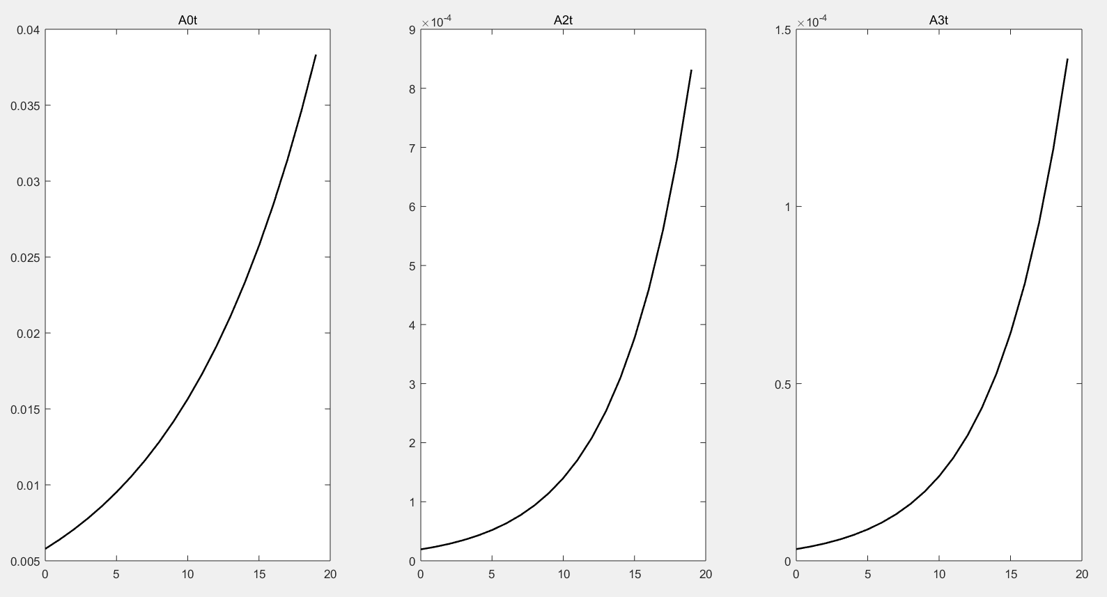
N=20;
x=0:N-1;
figure(1)
subplot (1,3,1)
plot(x,A0t(1:N),‘k’,‘LineWidth’,1.5)
subplot (1,3,2)
plot(x,A2t(1:N),‘k’,‘LineWidth’,1.5)
subplot (1,3,3)
plot(x,A3t(1:N),‘k’,‘LineWidth’,1.5)
The initial values were 121.3, 7693, and 1311, and the results start from 0.0058, 1.9316e-5, and 3.2918e-6.
The last(end) value is the same(121.3, 7693, 1311).
Do you know what the reason is?
@mrchae, I do not understand hat you are trying to do here. I do not know your model but if TFP is a state variable in your model you should write the equation as a_t = \rho a_{t-1} (note the difference in timing). Also the autoregressive parameters should be smaller that one in that case, otherwise the processes will be explosive…
What you are doing here, is that you consider TFP as a non predetermined variable. In this case it is correct to have an autoregressive parameter greater than one (see my recent post: The rank condition is verified. Eigenvalues are larger than 1). Setting A0t equal to 121.3 in the initval block you then ask Dynare (with the simul command) to compute a path for A0t such that the terminal condition is 121.3 (Dynare looks for an initial condition such that the iterations on the first equation is such that the terminal condition is equal to 121.3). I am not sure this what you… You probably need to read the manual (sections about deterministic simulations).
Best,
Stéphane.
Professor, thanks for easily explaining.
I realized that I was ignorant.
I just wonder how results would change when it was shocked.
var E_t, E_{1,t}, E_{2,t}, E_{3,t}, A_{2,t}, A_{3,t};
varexo \lambda;
parameters \alpha(=0.3), \beta(=0.985^{10}), \nu(=0.04), k_1(=0.5), k_2(=0.09), k_3(=0.41);
model;
E_t = (k_1 E_{1,t}^\rho + k_t E_{2,t}^\rho + k_3 E_{3,t}^\rho)^{1/\rho};
\frac{\nu k_1}{E_{1,t+1}^{1-\rho}E_{t+1}^{1-\rho}} - \lambda = \frac{1}{\beta}\bigg[\frac{\nu k_1}{E_{1,t}^{1-\rho}E_{t}^{1-\rho}} - \lambda\bigg];
A_{2,t}\bigg[\frac{\nu k_2}{E_{2,t}^{1-\rho}E_{t}^{1-\rho}} - \lambda\bigg] = 1 - \alpha - \nu;
A_{3,t}\frac{\nu k_3}{E_{3,t}^{1-\rho}E_{t}^{1-\rho}} = 1 - \alpha - \nu;
A_{2,t+1} = 1.02^{10} * A_{2,t};
A_{3,t+1} = 1.02^{10} * A_{3,t};
initial value
E_{1,0} = 39;
A_{2,0} = 7693;
A_{3,0} = 1311;
terminal condition
\lambda = 8*10^{-5};
simul(periods=20);
shocks;
val \lambda;
periods 1;
values 0;
ends;
Is it impossible?
I considered \lambda as a shock.
I wanted to see the change when \lambda was 0 in period 1 and changed to 8*10^{-5} from period 2 .
Best regards.
Sorry but it is very hard to understand what you write here, or your question. You should not mix latex symbols with what is supposed to be the content of a mod file. Even without understanding what you are looking for, the last block looks weird. The default value of a shock is zero, so there is no point in setting \lambda equal to zero in period 1. Also I do not understand how you specify the terminal condition.
Best,
Stéphane.
Thanks for reply, professor.
I’m sorry that I made the expression strange.
A simple version of my model is as follow.
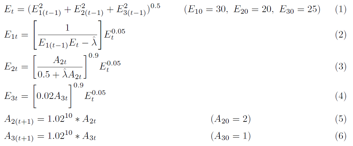
\hat{\lambda} = 0 in period 1~10.
\hat{\lambda} = 0.5 after period 10.
(Permanent increase in \hat{\lambda} at t=10)
I want to see the changes of E_t, E_{1t}, E_{2t}, and E_{3t} when the shock(\hat{\lambda}) comes.
Is it possible?
I wonder if it is possible to find a steady state with growth rate.
It’s very difficult for me.
Thanks for helping.
Best regards.
Sorry but I still do not understand your model… And I am not sure that you understand what is going on here. You have two forward looking variables A_2 and A_3, and I do not see how you can pin down the initial levels of these variables… Even if you add some terminal conditions for these variables, they are exogenous (w.r.t the rest of the model) and will not be affected by the shock \lambda. Hence there is no point in considering expected shock on \lambda. You probably should first read about DSGE and perfect foresight models…
Best,
Stéphane.
Thank you very much, professor.
I will try to study more.
It is a DSGE model in paper, but it’s difficult to apply to perfect foresight model.
Thanks again.
Best regards.