Hello everyone,
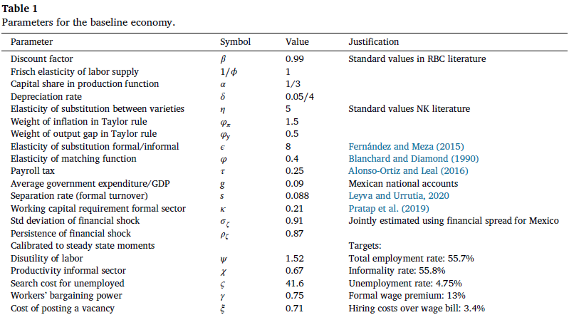
I am trying to replicate the “Does informality facilitate inflation stability?” by E. Alberola and C. Urrutia. To calibrate some parameters, they establish five targets:
Total employment rate: 0.557,
Informality rate: 0.558,
Unemployment rate: 0.0475,
Formal wage premium: 0.13,
Hiring costs over wage bill: 0.034.
I don’t understand what the authors mean by “hiring costs,” without this concept, it is difficult for me to establish a steady-state in terms of the parameters.
What I did was use the calibrated values and the targets (which I knew I was not going to get residuals equal to zero because of the omitted decimals in the paper) and trying to get the hiring cost over wage bill equal to 0.034, and the closest was the following:
They define the value of a match in the formal sector as
J_{t}^f = [p_{t}^f A_{t}^f - (1 + \kappa i_{t}^l + \tau) w_{t} ^f ] \lambda^C_{t} + \beta (1 - s) E\{ J_{t+1}^f \}
where J_{t}^f captures the value for an entrepreneur of keeping a match. Therefore, I think that hiring costs over wage bills are given by:
\frac{ [p_{t}^f A_{t}^f - (1 + \kappa i_{t}^l + \tau) w_{t} ^f ] \lambda^C_{t} }{w^f_{t}}
Which using the calibrated parameters of the paper is approximately 0.030. Is this correct?
I guess the only way to be sure is to ask the authors.
I managed to find the replica files and was able to deduce what the author means by hiring costs over wage bills. This is:
\frac{\xi V^f_{ss}}{w^f_{ss}L^f_{ss}} = 0.034,
where \xi are the vacancy posting costs, and V^f_{ss} are the vacancies.
But another problem arises. I am trying to translate this model to a weekly or fortnightly model, trying to keep the first 5 moments that the author proposes. I suppose that the first four are maintained in different periodicities, however, I have doubts about the last one since when leaving it as it is, the model cannot find the steady-state.
For the weekly model, modify the following parameters:
\beta_W = \beta^{1/12}, discount factor weekly
\delta_W = \delta/12, depreciation rate weekly
s_W = s/12, separation rate weekly
\vartheta_W = 12 \vartheta, Investment adjustment costs***
\theta_W = 1 - \frac{1 - \theta}{12}, Calvo parameter
Attached is an image of the calibrated parameters.
*** I did this because I found a topic in this forum that talked about adjustment costs in different time periods, however, In this paper the author handles capital adjustment costs, these are:
\Phi(\frac{I_{t}}{K_{t}}) = \frac{\vartheta}{2}(\frac{I_{t}}{K_{t}} - \delta)^2 K_{t}
I doubt that the parameter that measures the capital adjustment costs will have to be multiplied by 12, but I don’t know how to deal with this parameter, so my solution was to change the function to the investment adjustment costs.
My main question is: how to deal with the calibration target (V) (hiring costs over wag bills) on a weekly basis? In addition, to know if my intuition is correct that the rest of the calibration targets are maintained unchanged in different temporalities.
Thanks in advance.
As long as you are not dealing with the ratio of flows to stocks, there should be no aggregation issues. Both the costs and the wage bill are flows per period, whose ratio is unaffected if you aggregated them to lower frequency, e.g. multiply by 12 or so.
I really appreciate your response. I left the five calibration targets, however, the Fsolve file was not able to find the steady-state on a weekly basis, but on a fortnightly basis, so I will use this frequency for my model.
Finally, based on your experience, how do you deal with the capital adjustment cost parameter? My intuition is that by containing the quadratic investment capital ratio (and this is modified for different Flow/Stock periods), this parameter remains unchanged.
I think there are essentially 2 ways to proceed:
- You target actual moments in the data and adjust the parameter accordingly. I am not aware of a straightforward mapping here, so it would involve trial and error.
- Sometimes, you can target things like the elasticity of the investment to capital ratio with respect to Tobin’s q. An example would be DSGE_mod/Jermann1998_Algebra.pdf at master · JohannesPfeifer/DSGE_mod · GitHub (see Section 5)
1 Like