Bayesian Data for a Fiscal RBC Model

[riliatus]

Hi professor Pfeifer, after reading the first part of your paper “A Guide to Specifying Observation Equations for the Estimation of DSGE Models”, I’ve noticed that you used data from FRED, although, I tried to replicate a similar model (specificly, the one proposed as an exercise on the ‘Dynare Summer School 2021’) with my own data (for U.S from 1970-2019) to estimate that model, but it seems that my data isn’t appropiate (it isn’t able to execute the Bayesian Estimation). I’d like to know how did you obtained the data cointained in the file ‘ps_data.mat’ (i.e which variables do I have to look for in FRED database in order to calculare those per capita variables and specially the taxation rates for capital and labour).

Find attached the mod file and the mat files (‘data_usa’ is mine and ‘ps_data’ is your data).

Kind regards.

data_usa.mat (8.0 KB)
ps_data.mat (8.4 KB)
RBC_tax_estimation.mod (8.6 KB)

[jpfeifer]

Essentially, these are the tax rates described in Fiscal news and macroeconomic volatility - ScienceDirect and Policy risk and the business cycle - ScienceDirect

What is the problem in your estimation?

[riliatus]

Thanks, I’ll check those articles. Basically, I collected the data from FRED St. Louis (mnemonics in brackets) as stated in Pfeifer (2013), and given that the model is in per-capita terms, I estimated Y (FRED:GDPC1), C (FRED:PCE) and G (FRED:W068RCQ027SBEA) divided into N (FRED:CLF16OV) and then detrend the first log difference of those. Initially, I only used those 3 variables of mine, combined with your tax rates, and it results on this error message (find attached the .log file, error goes from line 720 to 775):

POSTERIOR KERNEL OPTIMIZATION PROBLEM!
(minus) the hessian matrix at the “mode” is not positive definite!
=> posterior variance of the estimated parameters are not positive.
You should try to change the initial values of the parameters using
the estimated_params_init block, or use another optimization routine.

RESULTS FROM POSTERIOR ESTIMATION
parameters
prior mean mode s.d. prior pstdev

rhoz 0.700 0.9960 NaN beta 0.1000
rhog 0.700 0.9416 NaN beta 0.1000
rho_n 0.700 0.9822 NaN beta 0.1000
rho_k 0.700 0.9266 NaN beta 0.1000

standard deviation of shocks
prior mean mode s.d. prior pstdev

eps_z 0.010 0.0052 NaN invg 0.1000
eps_g 0.010 0.0110 NaN invg 0.1000
eps_tk 0.010 0.0081 NaN invg 0.1000
eps_tn 0.010 0.0051 NaN invg 0.1000

standard deviation of measurement errors
prior mean mode s.d. prior pstdev

y_obs 0.010 0.0101 NaN invg 0.1000

Log data density [Laplace approximation] is NaN.

Note that the .mod file is unchanged and runs smoothly with ‘ps_data.mat’, but not with mine (‘data_usa’), either using only these 3 variables combined with your tax rates, or using your data for Y, C and G and my estimated tax rates.

Thanks and hope you can guide me with that issue.

RBC_tax_estimation.log (33.6 KB)

[jpfeifer]

You may need prior_trunc=0 and mode_compute=5.

[riliatus]

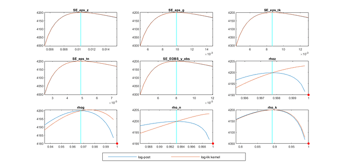
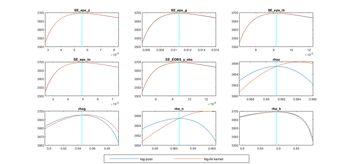
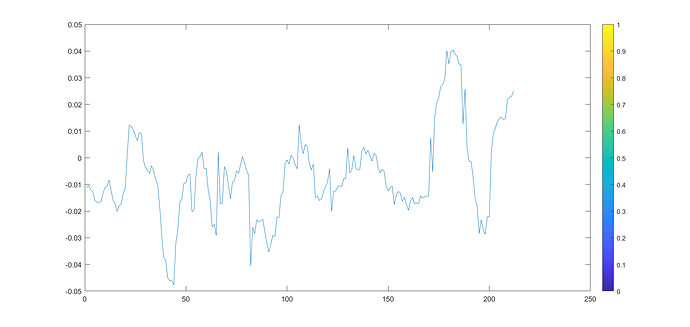
Well, it seems that the parameter prior_trunc=0 actually helped, however, mode_compute=5 was the default one in the .mod that I sent, so I changed it to mode_compute=6 and it worked (generated the trace plots, prior and posterior graphs, etc). But now I’ve estimated again the data based on Fiscal news and macroeconomic volatility - ScienceDirect and the original data (ps_data.mat) it’s similar to the new one (data_us.mat, figure 1), even the smoothed shocks and the “historical and smoothed variables” are, and when I run the .mod with this new dataset (which now it goes from 1959Q1 to 2021Q2) and with mode_compute=5 doesn’t, and with mode_compute=6 it actually seems to work, nevertheless, checking the “Mode Check Plot” there’re some red dots at the lower right corner (figure 2). I’d like to know why is this caused (I also attach the same plot that is generated but with the original dataset ps_data.mat, figure 3), does it means that it doesen’t converge or even that it isn’t an actual mode? Thanks.

Figure 1. ‘ps_data.mat tau_n’ - ‘data_us.mat tau_n’.

Figure 2. Mode Check Plot of the estimation with ‘data_us’ (mine).

Figure 3. Mode Check Plot of the estimation with ‘ps_data’ (the estimation works smoothly with this one).

[jpfeifer]

The red dots are for parameter values where the model has a problem. Here, it is obvious: in case of a unit (\rho=1) the Blanchard-Kahn conditions will not be satisfied.

[riliatus]

Okay I see. After doing some changes it works, now I included a consumption tax rate \tau^C_t, and after doing the math I was estimating the model as before, now including that tax rate as an observed variable, so I have two questions:

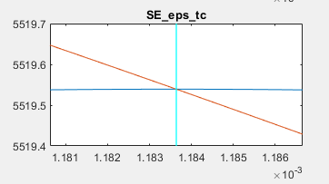
1. Which value should I use for the consumption tax shock variance (\varepsilon_{\tau_c}) in the shocks block (I’m still doing it for US data). I tried a value of \varepsilon_{\tau_c} = 0.0010^2 but it displayed an error and then tried with 0.0020^2, but the mode check plot for its standard error looked strange (figure 1).

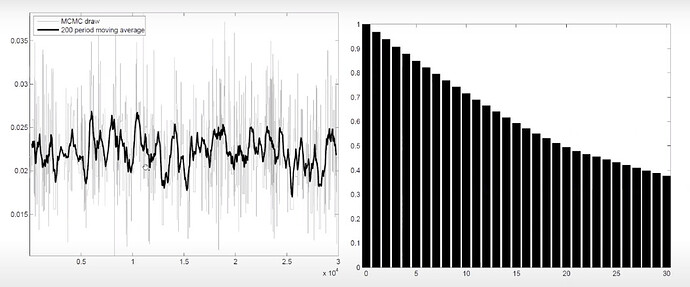
2. Is there any way to plot the autocorrelation histogram plot with the trace plot as the example in figure 2.

Thanks again.

Figure 1. Mode check plot for the standard error of \varepsilon_{\tau_c}

Figure 2. Trace and autocorrelation histogram plot.

[jpfeifer]

1. Do you want to calibrate or estimate it?
2. Have a look at Pfeifer (2014): “An Introduction to Graphs in Dynare”. The respective commands are documented there. If the question is how to show them next to each other in a PDF, the answer is that you have to do it manually.